Chapter 25 Elastic Net
We again use the Hitters dataset from the ISLR package to explore another shrinkage method, elastic net, which combines the ridge and lasso methods from the previous chapter.
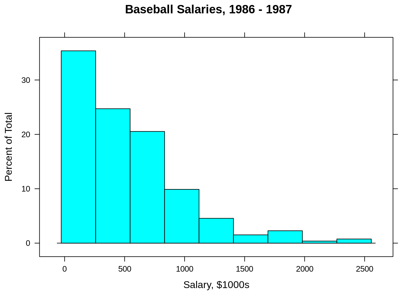
We again remove the missing data, which was all in the response variable, Salary.
## # A tibble: 263 x 20
##    AtBat  Hits HmRun  Runs   RBI Walks Years CAtBat CHits CHmRun CRuns  CRBI
##    <int> <int> <int> <int> <int> <int> <int>  <int> <int>  <int> <int> <int>
##  1   315    81     7    24    38    39    14   3449   835     69   321   414
##  2   479   130    18    66    72    76     3   1624   457     63   224   266
##  3   496   141    20    65    78    37    11   5628  1575    225   828   838
##  4   321    87    10    39    42    30     2    396   101     12    48    46
##  5   594   169     4    74    51    35    11   4408  1133     19   501   336
##  6   185    37     1    23     8    21     2    214    42      1    30     9
##  7   298    73     0    24    24     7     3    509   108      0    41    37
##  8   323    81     6    26    32     8     2    341    86      6    32    34
##  9   401    92    17    49    66    65    13   5206  1332    253   784   890
## 10   574   159    21   107    75    59    10   4631  1300     90   702   504
## # … with 253 more rows, and 8 more variables: CWalks <int>, League <fct>,
## #   Division <fct>, PutOuts <int>, Assists <int>, Errors <int>, Salary <dbl>,
## # NewLeague <fct>## [1] 263 20Because this dataset isn’t particularly large, we will forego a test-train split, and simply use all of the data as training data.
Since he have loaded caret, we also have access to the lattice package which has a nice histogram function.
25.1 Regression
Like ridge and lasso, we again attempt to minimize the residual sum of squares plus some penalty term.
\[ \sum_{i=1}^{n} \left( y_i - \beta_0 - \sum_{j=1}^{p} \beta_j x_{ij} \right) ^ 2 + \lambda\left[(1-\alpha)||\beta||_2^2/2 + \alpha ||\beta||_1\right] \]
Here, \(||\beta||_1\) is called the \(l_1\) norm.
\[ ||\beta||_1 = \sum_{j=1}^{p} |\beta_j| \] Similarly, \(||\beta||_2\) is called the \(l_2\), or Euclidean norm.
\[ ||\beta||_2 = \sqrt{\sum_{j=1}^{p} \beta_j^2} \]
These both quantify how “large” the coefficients are. Like lasso and ridge, the intercept is not penalized and glment takes care of standardization internally. Also reported coefficients are on the original scale.
The new penalty is \(\frac{\lambda \cdot (1-\alpha)}{2}\) times the ridge penalty plus \(\lambda \cdot \alpha\) times the lasso lasso penalty. (Dividing the ridge penalty by 2 is a mathematical convenience for optimization.) Essentially, with the correct choice of \(\lambda\) and \(\alpha\) these two “penalty coefficients” can be any positive numbers.
Often it is more useful to simply think of \(\alpha\) as controlling the mixing between the two penalties and \(\lambda\) controlling the amount of penalization. \(\alpha\) takes values between 0 and 1. Using \(\alpha = 1\) gives the lasso that we have seen before. Similarly, \(\alpha = 0\) gives ridge. We used these two before with glmnet() to specify which to method we wanted. Now we also allow for \(\alpha\) values in between.
We first setup our cross-validation strategy, which will be 5 fold. We then use train() with method = "glmnet" which is actually fitting the elastic net.
First, note that since we are using caret() directly, it is taking care of dummy variable creation. So unlike before when we used glmnet(), we do not need to manually create a model matrix.
Also note that we have allowed caret to choose the tuning parameters for us.
## glmnet
##
## 263 samples
##  19 predictor
##
## No pre-processing
## Resampling: Cross-Validated (5 fold)
## Summary of sample sizes: 211, 210, 210, 211, 210
## Resampling results across tuning parameters:
##
##   alpha  lambda   RMSE   Rsquared  MAE
##   0.10    0.5106  335.1  0.4549    235.2
##   0.10    5.1056  332.4  0.4632    231.9
##   0.10   51.0564  339.4  0.4486    231.1
##   0.55    0.5106  334.9  0.4551    234.5
##   0.55    5.1056  332.7  0.4650    230.4
##   0.55   51.0564  343.5  0.4440    235.9
##   1.00    0.5106  334.9  0.4546    234.1
##   1.00    5.1056  336.0  0.4590    230.6
##   1.00   51.0564  353.3  0.4231    244.1
##
## RMSE was used to select the optimal model using the smallest value.
## The final values used for the model were alpha = 0.1 and lambda = 5.106.
Notice a few things with these results. First, we have tried three \(\alpha\) values, 0.10, 0.55, and 1. It is not entirely clear why caret doesn’t use 0. It likely uses 0.10 to fit a model close to ridge, but with some potential for sparsity.
Here, the best result uses \(\alpha = 0.10\), so this result is somewhere between ridge and lasso, but closer to ridge.
hit_elnet_int = train(
  Salary ~ . ^ 2, data = Hitters,
  method = "glmnet",
  trControl = cv_5,
  tuneLength = 10
)
Now we try a much larger model search. First, we’re expanding the feature space to include all interactions. Since we are using penalized regression, we don’t have to worry as much about overfitting. If many of the added variables are not useful, we will likely use a model close to lasso which makes many of them 0.
We’re also using a larger tuning grid. By setting tuneLength = 10, we will search 10 \(\alpha\) values and 10 \(\lambda\) values for each. Because of this larger tuning grid, the results will be very large.
To deal with this, we write a quick helper function to extract the row with the best tuning parameters.
get_best_result = function(caret_fit) {
  best = which(rownames(caret_fit$results) == rownames(caret_fit$bestTune))
  best_result = caret_fit$results[best, ]
  rownames(best_result) = NULL
  best_result
}
We then call this function on the trained object.
##   alpha lambda  RMSE Rsquared   MAE RMSESD RsquaredSD MAESD
## 1     1  9.552 308.6   0.5555 209.5  55.16    0.08669 21.13
We see that the best result uses \(\alpha = 1\), which makes since. With \(\alpha = 1\), many of the added interaction coefficients are likely set to zero. (Unfortunately, obtaining this information after using caret with glmnet isn’t easy. The two don’t actually play very nice together. We’ll use cv.glmnet() with the expanded feature space to explore this.)
Also, this CV-RMSE is better than the lasso and ridge from the previous chapter that did not use the expanded feature space.
We also perform a quick analysis using cv.glmnet() instead. Due in part to randomness in cross validation, and differences in how cv.glmnet() and train() search for \(\lambda\), the results are slightly different.
set.seed(42)
X = model.matrix(Salary ~ . ^ 2, Hitters)[, -1]
y = Hitters$Salary

fit_lasso_cv = cv.glmnet(X, y, alpha = 1)
sqrt(fit_lasso_cv$cvm[fit_lasso_cv$lambda == fit_lasso_cv$lambda.min]) # CV-RMSE minimum
## [1] 306.9The commented line is not run, since it produces a lot of output, but if run, it will show that the fast majority of the coefficients are zero! Also, you’ll notice that cv.glmnet() does not respect the usual predictor hierarchy. Not a problem for prediction, but a massive interpretation issue!
## [1] 8## [1] 18325.2 Classification
Above, we have performed a regression task. But like lasso and ridge, elastic net can also be used for classification by using the deviance instead of the residual sum of squares. This essentially happens automatically in caret if the response variable is a factor.
We’ll test this using the familiar Default dataset, which we first test-train split.
set.seed(42)
default_idx = createDataPartition(Default$default, p = 0.75, list = FALSE)
default_trn = Default[default_idx, ]
default_tst = Default[-default_idx, ]
We then fit an elastic net with a default tuning grid.
## glmnet
##
## 7501 samples
##    3 predictor
##    2 classes: 'No', 'Yes'
##
## No pre-processing
## Resampling: Cross-Validated (5 fold)
## Summary of sample sizes: 6001, 6001, 6001, 6000, 6001
## Resampling results across tuning parameters:
##
##   alpha  lambda     Accuracy  Kappa
##   0.10   0.0001253  0.9732    0.41637
##   0.10   0.0012527  0.9727    0.37280
##   0.10   0.0125270  0.9676    0.07238
##   0.55   0.0001253  0.9735    0.42510
##   0.55   0.0012527  0.9727    0.38012
##   0.55   0.0125270  0.9679    0.09251
##   1.00   0.0001253  0.9736    0.42638
##   1.00   0.0012527  0.9725    0.38888
##   1.00   0.0125270  0.9692    0.16987
##
## Accuracy was used to select the optimal model using the largest value.
## The final values used for the model were alpha = 1 and lambda = 0.0001253.
Since the best model used \(\alpha = 1\), this is a lasso model.
We also try an expanded feature space, and a larger tuning grid.
def_elnet_int = train(
  default ~ . ^ 2, data = default_trn,
  method = "glmnet",
  trControl = cv_5,
  tuneLength = 10
)
Since the result here will return 100 models, we again use are helper function to simply extract the best result.
##   alpha   lambda Accuracy  Kappa AccuracySD KappaSD
## 1     1 0.001904   0.9732 0.4039   0.002846 0.07694
Here we see \(\alpha = 0.1\), which is a mix, but close to ridge.
Evaluating the test accuracy of this model, we obtain one of the highest accuracies for this dataset of all methods we have tried.
# test acc
calc_acc(actual = default_tst$default,
         predicted = predict(def_elnet_int, newdata = default_tst))
## [1] 0.973625.3 External Links
glmnetWeb Vingette - Details from the package developers.glmnetwithcaret- Some details on Elastic Net tuning in thecaretpackage.
25.4 rmarkdown
The rmarkdown file for this chapter can be found here. The file was created using R version 4.0.2. The following packages (and their dependencies) were loaded when knitting this file:
## [1] "glmnet" "Matrix" "caret" "ggplot2" "lattice"