Chapter 20 Resampling
- NOTE: This chapter is currently be re-written and will likely change considerably in the near future. It is currently lacking in a number of ways mostly narrative.
In this chapter we introduce resampling methods, in particular cross-validation. We will highlight the need for cross-validation by comparing it to our previous approach, which was to simply set aside some “test” data that we used for evaluating a model fit using “training” data. We will now refer to these held-out samples as the validation data and this approach as the validation set approach. Along the way we’ll redefine the notion of a “test” dataset.
To illustrate the use of resampling techniques, we’ll consider a regression setup with a single predictor \(x\), and a regression function \(f(x) = x^3\). Adding an additional noise parameter, we define the entire data generating process as
\[ Y \sim N(\mu = x^3, \sigma^2 = 0.25 ^ 2) \]
We write an R function that generates datasets according to this process.
gen_sim_data = function(sample_size) {
  x = runif(n = sample_size, min = -1, max = 1)
  y = rnorm(n = sample_size, mean = x ^ 3, sd = 0.25)
  data.frame(x, y)
}
We first simulate a single dataset, which we also split into a train and validation set. Here, the validation set is 20% of the data.
set.seed(42)
sim_data = gen_sim_data(sample_size = 200)
sim_idx  = sample(1:nrow(sim_data), 160)
sim_trn  = sim_data[sim_idx, ]
sim_val  = sim_data[-sim_idx, ]
We plot this training data, as well as the true regression function.
plot(y ~ x, data = sim_trn, col = "dodgerblue", pch = 20)
grid()
curve(x ^ 3, add = TRUE, col = "black", lwd = 2)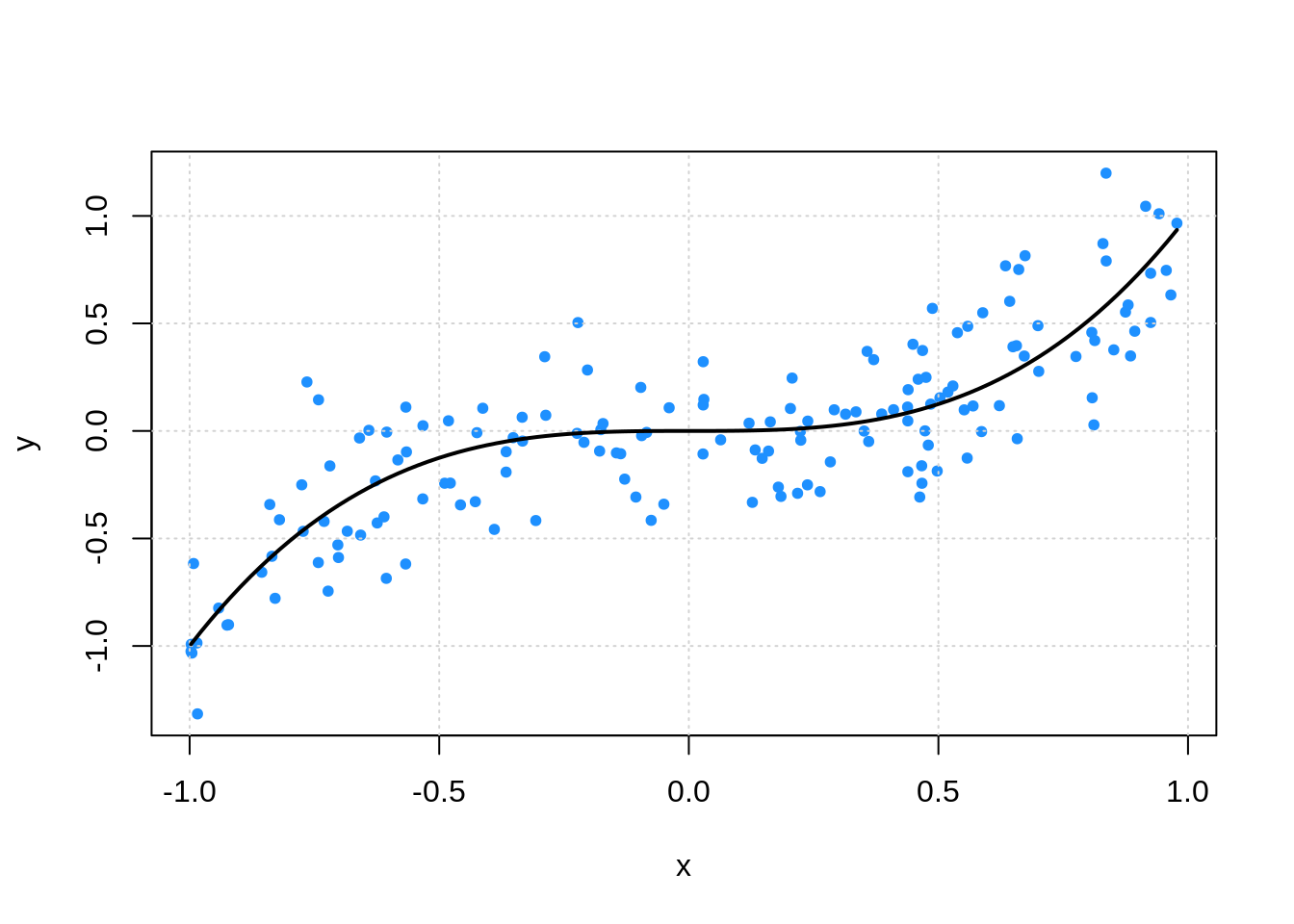
Recall that we needed this validation set because the training error was far too optimistic for highly flexible models. This would lead us to always use the most flexible model.
fit = lm(y ~ poly(x, 10), data = sim_trn)

calc_rmse(actual = sim_trn$y, predicted = predict(fit, sim_trn))
## [1] 0.2297774## [1] 0.277046220.1 Validation-Set Approach
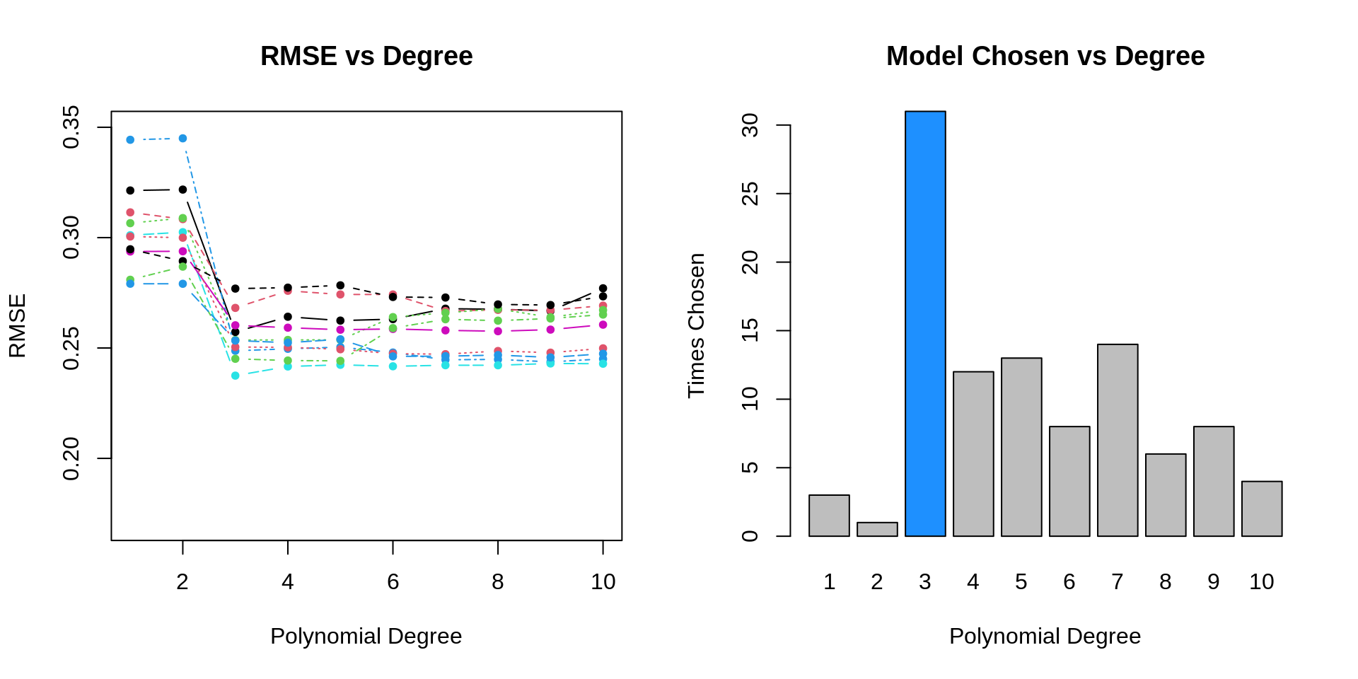
- TODO: consider fitting polynomial models of degree k = 1:10 to data from this data generating process
- TODO: here, we can consider k, the polynomial degree, as a tuning parameter
- TODO: perform simulation study to evaluate how well validation set approach works
- TODO: each simulation we will…
set.seed(42)
for (i in 1:num_sims) {
  # simulate data
  sim_data = gen_sim_data(sample_size = 200)
  # set aside validation set
  sim_idx = sample(1:nrow(sim_data), 160)
  sim_trn = sim_data[sim_idx, ]
  sim_val = sim_data[-sim_idx, ]
  # fit models and store RMSEs
  for (j in 1:num_degrees) {
    #fit model
    fit = glm(y ~ poly(x, degree = j), data = sim_trn)
    # calculate error
    val_rmse[i, j] = calc_rmse(actual = sim_val$y, predicted = predict(fit, sim_val))
  }
}
- TODO: issues are hard to “see” but have to do with variability
20.2 Cross-Validation
Instead of using a single test-train split, we instead look to use \(K\)-fold cross-validation.
\[ \text{RMSE-CV}_{K} = \sum_{k = 1}^{K} \frac{n_k}{n} \text{RMSE}_k \]
\[ \text{RMSE}_k = \sqrt{\frac{1}{n_k} \sum_{i \in C_k} \left( y_i - \hat{f}^{-k}(x_i) \right)^2 } \]
- \(n_k\) is the number of observations in fold \(k\)
- \(C_k\) are the observations in fold \(k\)
- \(\hat{f}^{-k}()\) is the trained model using the training data without fold \(k\)
If \(n_k\) is the same in each fold, then
\[ \text{RMSE-CV}_{K} = \frac{1}{K}\sum_{k = 1}^{K} \text{RMSE}_k \]
- TODO: create and add graphic that shows the splitting process
- TODO: Can be used with any metric, MSE, RMSE, class-err, class-acc
There are many ways to perform cross-validation in R, depending on the statistical learning method of interest. Some methods, for example glm() through boot::cv.glm() and knn() through knn.cv() have cross-validation capabilities built-in. We’ll use glm() for illustration. First we need to convince ourselves that glm() can be used to perform the same tasks as lm().
## (Intercept) poly(x, 3)1 poly(x, 3)2 poly(x, 3)3
## -0.0289307 4.5471322 -0.1527198 2.3895917## (Intercept) poly(x, 3)1 poly(x, 3)2 poly(x, 3)3
## -0.0289307 4.5471322 -0.1527198 2.3895917By default, cv.glm() will report leave-one-out cross-validation (LOOCV).
## [1] 0.2598565 0.2598342We are actually given two values. The first is exactly the LOOCV-MSE. The second is a minor correction that we will not worry about. We take a square root to obtain LOOCV-RMSE.
In practice, we often prefer 5 or 10-fold cross-validation for a number of reason, but often most importantly, for computational efficiency.
## [1] 0.2628287 0.2617056We repeat the above simulation study, this time performing 5-fold cross-validation. With a total sample size of \(n = 200\) each validation set has 40 observations, as did the single validation set in the previous simulations.
set.seed(42)
for (i in 1:num_sims) {
  # simulate data, use all data for training
  sim_trn = gen_sim_data(sample_size = 200)
  # fit models and store RMSE
  for (j in 1:num_degrees) {
    #fit model
    fit = glm(y ~ poly(x, degree = j), data = sim_trn)
    # calculate error
    cv_rmse[i, j] = sqrt(boot::cv.glm(sim_trn, fit, K = 5)$delta[1])
  }
}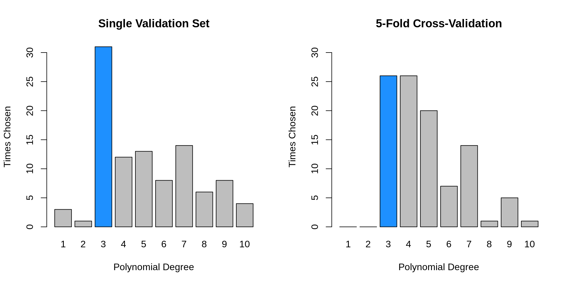
| Polynomial Degree | Mean, Val | SD, Val | Mean, CV | SD, CV |
|---|---|---|---|---|
| 1 | 0.290 | 0.031 | 0.293 | 0.015 |
| 2 | 0.291 | 0.031 | 0.295 | 0.014 |
| 3 | 0.247 | 0.027 | 0.251 | 0.010 |
| 4 | 0.248 | 0.028 | 0.252 | 0.010 |
| 5 | 0.248 | 0.027 | 0.253 | 0.010 |
| 6 | 0.249 | 0.027 | 0.254 | 0.011 |
| 7 | 0.251 | 0.027 | 0.255 | 0.012 |
| 8 | 0.252 | 0.027 | 0.257 | 0.011 |
| 9 | 0.253 | 0.028 | 0.258 | 0.012 |
| 10 | 0.255 | 0.027 | 0.259 | 0.012 |
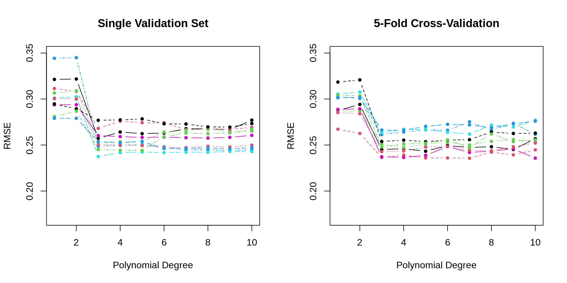
- TODO: differences: less variance, better selections
20.3 Test Data
The following example, inspired by The Elements of Statistical Learning, will illustrate the need for a dedicated test set which is never used in model training. We do this, if for no other reason, because it gives us a quick sanity check that we have cross-validated correctly. To be specific we will always test-train split the data, then perform cross-validation within the training data.
Essentially, this example will also show how to not cross-validate properly. It will also show can example of cross-validated in a classification setting.
Consider a binary response \(Y\) with equal probability to take values \(0\) and \(1\).
\[ Y \sim \text{bern}(p = 0.5) \]
Also consider \(p = 10,000\) independent predictor variables, \(X_j\), each with a standard normal distribution.
\[ X_j \sim N(\mu = 0, \sigma^2 = 1) \]
We simulate \(n = 100\) observations from this data generating process. Notice that the way we’ve defined this process, none of the \(X_j\) are related to \(Y\).
set.seed(42)
n = 200
p = 10000
x = replicate(p, rnorm(n))
y = c(rbinom(n = n, size = 1, prob = 0.5))
full_data = data.frame(y, x)
Before attempting to perform cross-validation, we test-train split the data, using half of the available data for each. (In practice, with this little data, it would be hard to justify a separate test dataset, but here we do so to illustrate another point.)
trn_idx  = sample(1:nrow(full_data), trunc(nrow(full_data) * 0.5))
trn_data = full_data[trn_idx,   ]
tst_data = full_data[-trn_idx, ]
Now we would like to train a logistic regression model to predict \(Y\) using the available predictor data. However, here we have \(p > n\), which prevents us from fitting logistic regression. To overcome this issue, we will first attempt to find a subset of relevant predictors. To do so, we’ll simply find the predictors that are most correlated with the response.
# find correlation between y and each predictor variable
correlations = apply(trn_data[, -1], 2, cor, y = trn_data$y)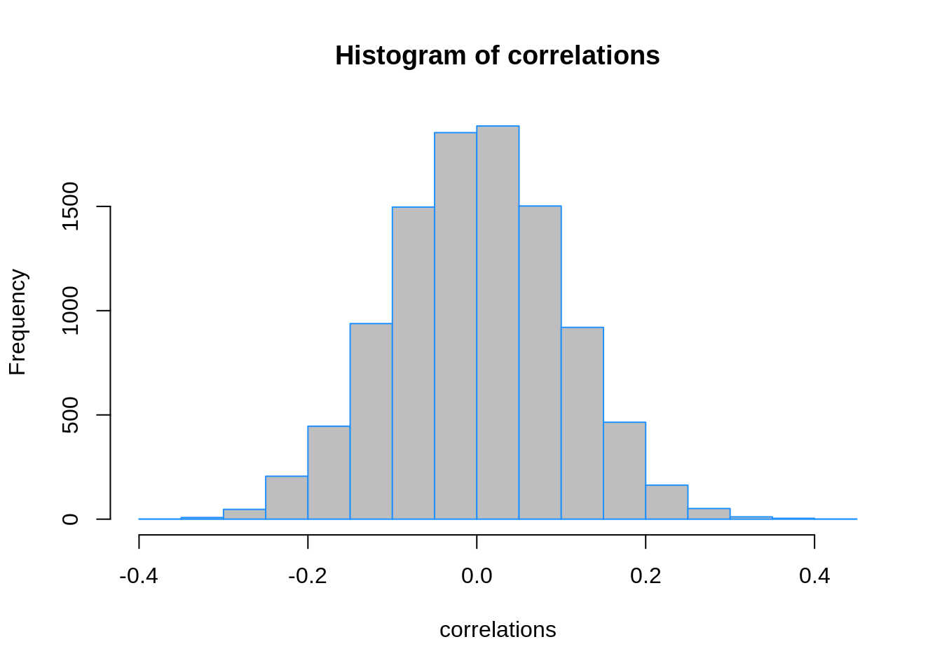
While many of these correlations are small, many very close to zero, some are as large as 0.40. Since our training data has 50 observations, we’ll select the 25 predictors with the largest (absolute) correlations.
##      X4942       X867      X8617      X8044       X406      X4358      X7725
##  0.4005771  0.3847397  0.3809371  0.3692479 -0.3571329  0.3553777 -0.3459522
##      X1986      X3784        X77      X7010      X9354      X8450      X2355
## -0.3448612  0.3298109 -0.3252776 -0.3242813  0.3227353  0.3220087  0.3192606
##      X4381      X2486      X5947      X5767      X1227      X1464      X8223
##  0.3157441  0.3149892  0.3131235  0.3114936 -0.3105052 -0.3104528  0.3084551
##       X188      X4203      X2234      X1098
##  0.3065491  0.3039848 -0.3036512 -0.3036153
We subset the training and test sets to contain only the response as well as these 25 predictors.
Then we finally fit an additive logistic regression using this subset of predictors. We perform 10-fold cross-validation to obtain an estimate of the classification error.
add_log_mod = glm(y ~ ., data = trn_screen, family = "binomial")
boot::cv.glm(trn_screen, add_log_mod, K = 10)$delta[1]
## [1] 0.3742339The 10-fold cross-validation is suggesting a classification error estimate of almost 30%.
add_log_pred = (predict(add_log_mod, newdata = tst_screen, type = "response") > 0.5) * 1
calc_err(predicted = add_log_pred, actual = tst_screen$y)
## [1] 0.48However, if we obtain an estimate of the error using the set, we see an error rate of 50%. No better than guessing! But since \(Y\) has no relationship with the predictors, this is actually what we would expect. This incorrect method we’ll call screen-then-validate.
Now, we will correctly screen-while-validating. Essentially, instead of simply cross-validating the logistic regression, we also need to cross validate the screening process. That is, we won’t simply use the same variables for each fold, we get the “best” predictors for each fold.
For methods that do not have a built-in ability to perform cross-validation, or for methods that have limited cross-validation capability, we will need to write our own code for cross-validation. (Spoiler: This is not completely true, but let’s pretend it is, so we can see how to perform cross-validation from scratch.)
This essentially amounts to randomly splitting the data, then looping over the splits. The createFolds() function from the caret() package will make this much easier.
## $Fold01
##  [1] 17 23 27 44 45 76 85 87 93 97
##
## $Fold02
##  [1]  6 14 15 26 37 38 55 68 69 71
##
## $Fold03
##  [1]  3  4  7 29 39 52 54 57 59 82
##
## $Fold04
##  [1] 19 21 40 46 48 56 73 78 91 96
##
## $Fold05
##  [1] 25 34 36 58 61 65 66 75 83 89
##
## $Fold06
##  [1]  2  9 10 62 74 79 80 90 92 98
##
## $Fold07
##  [1]  8 31 32 41 43 53 60 67 88 95
##
## $Fold08
##  [1] 12 18 33 35 42 49 51 64 84 94
##
## $Fold09
##  [1]  11  13  16  20  28  47  50  77  99 100
##
## $Fold10
##  [1]  1  5 22 24 30 63 70 72 81 86
# use the caret package to obtain 10 "folds"
folds = caret::createFolds(trn_data$y, k = 10)
# for each fold
# - pre-screen variables on the 9 training folds
# - fit model to these variables
# - get error on validation fold
fold_err = rep(0, length(folds))
for (i in seq_along(folds)) {
# split for fold i
trn_fold = trn_data[-folds[[i]], ]
val_fold = trn_data[folds[[i]], ]
# screening for fold i
correlations = apply(trn_fold[, -1], 2, cor, y = trn_fold[,1])
selected = order(abs(correlations), decreasing = TRUE)[1:25]
trn_fold_screen = trn_fold[ , c(1, selected)]
val_fold_screen = val_fold[ , c(1, selected)]
# error for fold i
add_log_mod = glm(y ~ ., data = trn_fold_screen, family = "binomial")
add_log_prob = predict(add_log_mod, newdata = val_fold_screen, type = "response")
add_log_pred = ifelse(add_log_prob > 0.5, yes = 1, no = 0)
fold_err[i] = mean(add_log_pred != val_fold_screen$y)
}
# report all 10 validation fold errors
fold_err## [1] 0.4 0.9 0.6 0.4 0.6 0.3 0.7 0.5 0.6 0.6# properly cross-validated error
# this roughly matches what we expect in the test set
mean(fold_err)## [1] 0.56- TODO: note that, even cross-validated correctly, this isn’t a brilliant variable selection procedure. (it completely ignores interactions and correlations among the predictors. however, if it works, it works.) next chapters…
20.4 Bootstrap
ISL discusses the bootstrap, which is another resampling method. However, it is less relevant to the statistical learning tasks we will encounter. It could be used to replace cross-validation, but encounters significantly more computation.
It could be more useful if we were to attempt to calculate the bias and variance of a prediction (estimate) without access to the data generating process. Return to the bias-variance tradeoff chapter and think about how the bootstrap could be used to obtain estimates of bias and variance with a single dataset, instead of repeated simulated datasets.
20.5 Which \(K\)?
- TODO: LOO vs 5 vs 10
- TODO: bias and variance
20.6 Summary
- TODO: using cross validation for: tuning, error estimation
20.7 External Links
- YouTube: Cross-Validation, Part 1 - Video from user “mathematicalmonk” which introduces \(K\)-fold cross-validation in greater detail.
- YouTube: Cross-Validation, Part 2 - Continuation which discusses selection and resampling strategies.
- YouTube: Cross-Validation, Part 3 - Continuation which discusses choice of \(K\).
- Blog: Fast Computation of Cross-Validation in Linear Models - Details for using leverage to speed-up LOOCV for linear models.
- OTexts: Bootstrap - Some brief mathematical details of the bootstrap.
20.8 rmarkdown
The rmarkdown file for this chapter can be found here. The file was created using R version 4.0.2.