Chapter 24 Regularization
Chapter Status: Currently this chapter is very sparse. It essentially only expands upon an example discussed in ISL, thus only illustrates usage of the methods. Mathematical and conceptual details of the methods will be added later. Also, more comments on using glmnet with caret will be discussed.
We will use the Hitters dataset from the ISLR package to explore two shrinkage methods: ridge regression and lasso. These are otherwise known as penalized regression methods.
This dataset has some missing data in the response Salaray. We use the na.omit() function the clean the dataset.
## [1] 59## [1] 59## [1] 0The predictors variables are offensive and defensive statistics for a number of baseball players.
##  [1] "AtBat"     "Hits"      "HmRun"     "Runs"      "RBI"       "Walks"
##  [7] "Years"     "CAtBat"    "CHits"     "CHmRun"    "CRuns"     "CRBI"
## [13] "CWalks"    "League"    "Division"  "PutOuts"   "Assists"   "Errors"
## [19] "Salary"    "NewLeague"
We use the glmnet() and cv.glmnet() functions from the glmnet package to fit penalized regressions.
Unfortunately, the glmnet function does not allow the use of model formulas, so we setup the data for ease of use with glmnet. Eventually we will use train() from caret which does allow for fitting penalized regression with the formula syntax, but to explore some of the details, we first work with the functions from glmnet directly.
First, we fit an ordinary linear regression, and note the size of the predictors’ coefficients, and predictors’ coefficients squared. (The two penalties we will use.)
##  (Intercept)        AtBat         Hits        HmRun         Runs          RBI
##  163.1035878   -1.9798729    7.5007675    4.3308829   -2.3762100   -1.0449620
##        Walks        Years       CAtBat        CHits       CHmRun        CRuns
##    6.2312863   -3.4890543   -0.1713405    0.1339910   -0.1728611    1.4543049
##         CRBI       CWalks      LeagueN    DivisionW      PutOuts      Assists
##    0.8077088   -0.8115709   62.5994230 -116.8492456    0.2818925    0.3710692
##       Errors   NewLeagueN
## -3.3607605 -24.7623251## [1] 238.7295## [1] 18337.324.1 Ridge Regression
We first illustrate ridge regression, which can be fit using glmnet() with alpha = 0 and seeks to minimize
\[ \sum_{i=1}^{n} \left( y_i - \beta_0 - \sum_{j=1}^{p} \beta_j x_{ij} \right) ^ 2 + \lambda \sum_{j=1}^{p} \beta_j^2 . \]
Notice that the intercept is not penalized. Also, note that that ridge regression is not scale invariant like the usual unpenalized regression. Thankfully, glmnet() takes care of this internally. It automatically standardizes predictors for fitting, then reports fitted coefficient using the original scale.
The two plots illustrate how much the coefficients are penalized for different values of \(\lambda\). Notice none of the coefficients are forced to be zero.
par(mfrow = c(1, 2))
fit_ridge = glmnet(X, y, alpha = 0)
plot(fit_ridge)
plot(fit_ridge, xvar = "lambda", label = TRUE)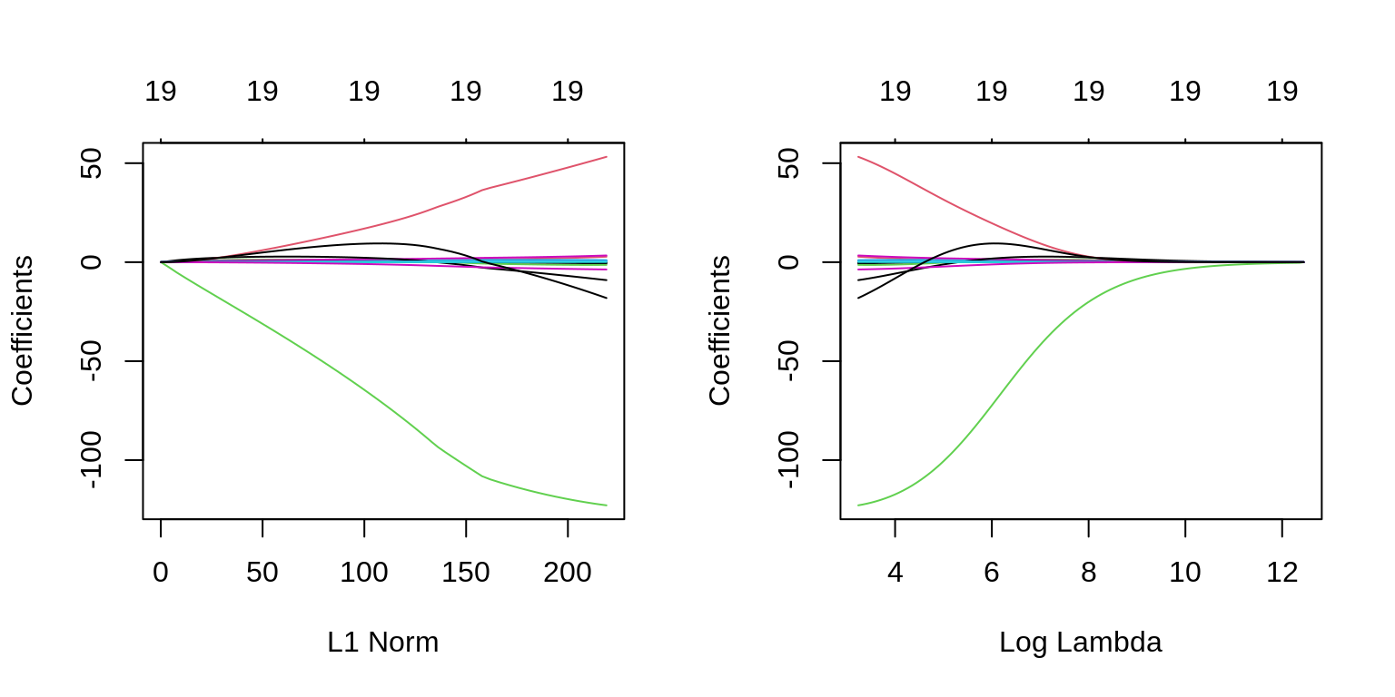
We use cross-validation to select a good \(\lambda\) value. The cv.glmnet()function uses 10 folds by default. The plot illustrates the MSE for the \(\lambda\)s considered. Two lines are drawn. The first is the \(\lambda\) that gives the smallest MSE. The second is the \(\lambda\) that gives an MSE within one standard error of the smallest.
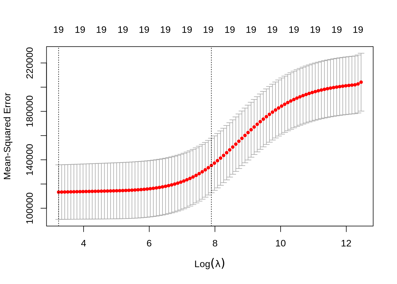
The cv.glmnet() function returns several details of the fit for both \(\lambda\) values in the plot. Notice the penalty terms are smaller than the full linear regression. (As we would expect.)
## 20 x 1 sparse Matrix of class "dgCMatrix"
##                         1
## (Intercept) 213.066444060
## AtBat         0.090095728
## Hits          0.371252755
## HmRun         1.180126954
## Runs          0.596298285
## RBI           0.594502389
## Walks         0.772525465
## Years         2.473494235
## CAtBat        0.007597952
## CHits         0.029272172
## CHmRun        0.217335715
## CRuns         0.058705097
## CRBI          0.060722036
## CWalks        0.058698830
## LeagueN       3.276567808
## DivisionW   -21.889942546
## PutOuts       0.052667119
## Assists       0.007463678
## Errors       -0.145121335
## NewLeagueN 2.972759111## 20 x 1 sparse Matrix of class "dgCMatrix"
## 1
## (Intercept) 8.112693e+01
## AtBat -6.815959e-01
## Hits 2.772312e+00
## HmRun -1.365680e+00
## Runs 1.014826e+00
## RBI 7.130225e-01
## Walks 3.378558e+00
## Years -9.066800e+00
## CAtBat -1.199478e-03
## CHits 1.361029e-01
## CHmRun 6.979958e-01
## CRuns 2.958896e-01
## CRBI 2.570711e-01
## CWalks -2.789666e-01
## LeagueN 5.321272e+01
## DivisionW -1.228345e+02
## PutOuts 2.638876e-01
## Assists 1.698796e-01
## Errors -3.685645e+00
## NewLeagueN -1.810510e+01## [1] 18367.29## 20 x 1 sparse Matrix of class "dgCMatrix"
## 1
## (Intercept) 213.066444060
## AtBat 0.090095728
## Hits 0.371252755
## HmRun 1.180126954
## Runs 0.596298285
## RBI 0.594502389
## Walks 0.772525465
## Years 2.473494235
## CAtBat 0.007597952
## CHits 0.029272172
## CHmRun 0.217335715
## CRuns 0.058705097
## CRBI 0.060722036
## CWalks 0.058698830
## LeagueN 3.276567808
## DivisionW -21.889942546
## PutOuts 0.052667119
## Assists 0.007463678
## Errors -0.145121335
## NewLeagueN 2.972759111## [1] 507.788## [1] 132355.6## [1] 451.8190 450.1773 449.3764 449.1046 448.8075 448.4828 448.1282 447.7410
## [9] 447.3185 446.8577 446.3555 445.8084 445.2128 444.5650 443.8610 443.0966
## [17] 442.2674 441.3691 440.3969 439.3462 438.2122 436.9901 435.6753 434.2633
## [25] 432.7497 431.1308 429.4030 427.5636 425.6103 423.5420 421.3583 419.0604
## [33] 416.6504 414.1319 411.5104 408.7927 405.9875 403.1047 400.1563 397.1558
## [41] 394.1178 391.0583 387.9941 384.9424 381.9207 378.9462 376.0354 373.2039
## [49] 370.4660 367.8342 365.3184 362.9276 360.6688 358.5458 356.5609 354.7144
## [57] 353.0045 351.4284 349.9815 348.6584 347.4528 346.3581 345.3671 344.4723
## [65] 343.6699 342.9507 342.3074 341.7328 341.2215 340.7696 340.3715 340.0189
## [73] 339.7092 339.4383 339.1988 338.9890 338.8065 338.6429 338.4985 338.3709
## [81] 338.2534 338.1472 338.0493 337.9563 337.8694 337.7825 337.6966 337.6125
## [89] 337.5297 337.4436 337.3577 337.2712 337.1844 337.0973 337.0109 336.9265
## [97] 336.8448 336.7658 336.6928 336.5957# CV-RMSE using minimum lambda
sqrt(fit_ridge_cv$cvm[fit_ridge_cv$lambda == fit_ridge_cv$lambda.min])## [1] 336.5957# CV-RMSE using 1-SE rule lambda
sqrt(fit_ridge_cv$cvm[fit_ridge_cv$lambda == fit_ridge_cv$lambda.1se]) ## [1] 367.834224.2 Lasso
We now illustrate lasso, which can be fit using glmnet() with alpha = 1 and seeks to minimize
\[ \sum_{i=1}^{n} \left( y_i - \beta_0 - \sum_{j=1}^{p} \beta_j x_{ij} \right) ^ 2 + \lambda \sum_{j=1}^{p} |\beta_j| . \]
Like ridge, lasso is not scale invariant.
The two plots illustrate how much the coefficients are penalized for different values of \(\lambda\). Notice some of the coefficients are forced to be zero.
par(mfrow = c(1, 2))
fit_lasso = glmnet(X, y, alpha = 1)
plot(fit_lasso)
plot(fit_lasso, xvar = "lambda", label = TRUE)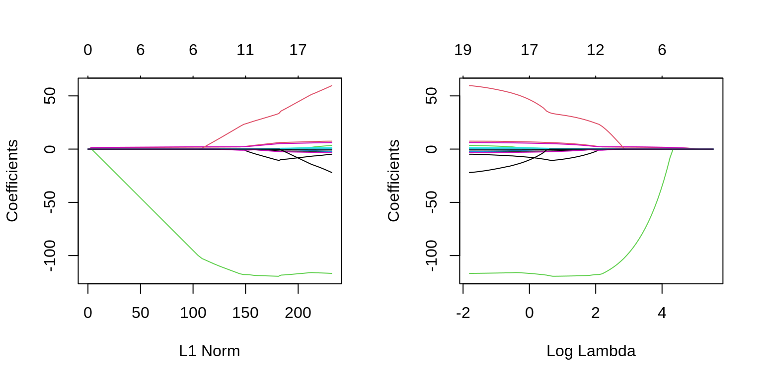
Again, to actually pick a \(\lambda\), we will use cross-validation. The plot is similar to the ridge plot. Notice along the top is the number of features in the model. (Which changed in this plot.)
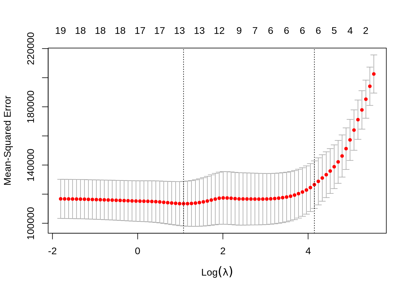
cv.glmnet() returns several details of the fit for both \(\lambda\) values in the plot. Notice the penalty terms are again smaller than the full linear regression. (As we would expect.) Some coefficients are 0.
## 20 x 1 sparse Matrix of class "dgCMatrix"
##                       1
## (Intercept) 115.3773591
## AtBat         .
## Hits          1.4753071
## HmRun         .
## Runs          .
## RBI           .
## Walks         1.6566947
## Years         .
## CAtBat        .
## CHits         .
## CHmRun        .
## CRuns         0.1660465
## CRBI          0.3453397
## CWalks        .
## LeagueN       .
## DivisionW   -19.2435215
## PutOuts       0.1000068
## Assists       .
## Errors        .
## NewLeagueN .## 20 x 1 sparse Matrix of class "dgCMatrix"
## 1
## (Intercept) 117.5258436
## AtBat -1.4742901
## Hits 5.4994256
## HmRun .
## Runs .
## RBI .
## Walks 4.5991651
## Years -9.1918308
## CAtBat .
## CHits .
## CHmRun 0.4806743
## CRuns 0.6354799
## CRBI 0.3956153
## CWalks -0.4993240
## LeagueN 31.6238173
## DivisionW -119.2516409
## PutOuts 0.2704287
## Assists 0.1594997
## Errors -1.9426357
## NewLeagueN .## [1] 15363.99## 20 x 1 sparse Matrix of class "dgCMatrix"
## 1
## (Intercept) 115.3773591
## AtBat .
## Hits 1.4753071
## HmRun .
## Runs .
## RBI .
## Walks 1.6566947
## Years .
## CAtBat .
## CHits .
## CHmRun .
## CRuns 0.1660465
## CRBI 0.3453397
## CWalks .
## LeagueN .
## DivisionW -19.2435215
## PutOuts 0.1000068
## Assists .
## Errors .
## NewLeagueN .## [1] 375.3911## [1] 116096.9## [1] 450.0450 440.5806 430.3877 421.7269 413.7075 404.9846 396.5670 388.9057
## [9] 382.3740 377.0449 372.5904 368.6293 365.1786 362.0757 358.8760 355.7098
## [17] 352.8639 350.4950 348.5285 346.8972 345.4898 344.3528 343.5417 342.9243
## [25] 342.4168 342.0202 341.7265 341.5692 341.5012 341.4663 341.5029 341.5574
## [33] 341.5857 341.6196 341.6445 341.9246 342.3273 342.5799 342.6550 342.3637
## [41] 341.5039 340.5235 339.5177 338.6793 337.9687 337.4356 337.0628 336.8681
## [49] 336.8258 336.8874 337.2062 337.5072 337.8550 338.2128 338.6038 338.8880
## [57] 339.0800 339.2685 339.3322 339.4100 339.5017 339.6380 339.8072 339.9620
## [65] 340.1314 340.2814 340.4493 340.5705 340.7112 340.8467 340.9535 341.0781
## [73] 341.2051 341.3688 341.4405 341.4999 341.5540 341.6055 341.6554 341.7065# CV-RMSE using minimum lambda
sqrt(fit_lasso_cv$cvm[fit_lasso_cv$lambda == fit_lasso_cv$lambda.min])## [1] 336.8258# CV-RMSE using 1-SE rule lambda
sqrt(fit_lasso_cv$cvm[fit_lasso_cv$lambda == fit_lasso_cv$lambda.1se]) ## [1] 355.709824.3 broom
Sometimes, the output from glmnet() can be overwhelming. The broom package can help with that.
library(broom)
# the output from the commented line would be immense
# fit_lasso_cv
tidy(fit_lasso_cv)
## # A tibble: 80 x 6
## lambda estimate std.error conf.low conf.high nzero
## <dbl> <dbl> <dbl> <dbl> <dbl> <int>
## 1 255. 202540. 13105. 189435. 215646. 0
## 2 233. 194111. 13163. 180948. 207274. 1
## 3 212. 185234. 13087. 172146. 198321. 2
## 4 193. 177854. 13190. 164664. 191043. 2
## 5 176. 171154. 13498. 157655. 184652. 3
## 6 160. 164013. 13875. 150137. 177888. 4
## 7 146. 157265. 14093. 143172. 171359. 4
## 8 133. 151248. 14277. 136971. 165525. 4
## 9 121. 146210. 14481. 131728. 160691. 4
## 10 111. 142163. 14731. 127432. 156894. 4
## # … with 70 more rows## # A tibble: 1 x 3
## lambda.min lambda.1se nobs
## <dbl> <dbl> <int>
## 1 2.94 63.2 26324.4 Simulated Data, \(p > n\)
Aside from simply shrinking coefficients (ridge) and setting some coefficients to 0 (lasso), penalized regression also has the advantage of being able to handle the \(p > n\) case.
set.seed(1234)
n = 1000
p = 5500
X = replicate(p, rnorm(n = n))
beta = c(1, 1, 1, rep(0, 5497))
z = X %*% beta
prob = exp(z) / (1 + exp(z))
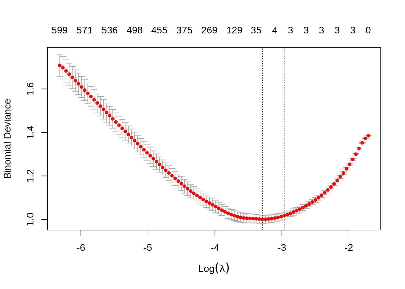
y = as.factor(rbinom(length(z), size = 1, prob = prob))We first simulate a classification example where \(p > n\).
We then use a lasso penalty to fit penalized logistic regression. This minimizes
\[ \sum_{i=1}^{n} L\left(y_i, \beta_0 + \sum_{j=1}^{p} \beta_j x_{ij}\right) + \lambda \sum_{j=1}^{p} |\beta_j| \]
where \(L\) is the appropriate negative log-likelihood.
## 10 x 1 sparse Matrix of class "dgCMatrix"
##                      1
## (Intercept) 0.02397452
## V1          0.59674958
## V2          0.56251761
## V3          0.60065105
## V4          .
## V5          .
## V6          .
## V7          .
## V8          .
## V9 .## s0 s1 s2 s3 s4 s5 s6 s7 s8 s9 s10 s11 s12 s13 s14 s15 s16 s17 s18 s19
## 0 2 3 3 3 3 3 3 3 3 3 3 3 3 3 3 3 3 3 3
## s20 s21 s22 s23 s24 s25 s26 s27 s28 s29 s30 s31 s32 s33 s34 s35 s36 s37 s38 s39
## 3 3 3 3 3 3 3 3 3 3 4 6 7 10 18 24 35 54 65 75
## s40 s41 s42 s43 s44 s45 s46 s47 s48 s49 s50 s51 s52 s53 s54 s55 s56 s57 s58 s59
## 86 100 110 129 147 168 187 202 221 241 254 269 283 298 310 324 333 350 364 375
## s60 s61 s62 s63 s64 s65 s66 s67 s68 s69 s70 s71 s72 s73 s74 s75 s76 s77 s78 s79
## 387 400 411 429 435 445 453 455 462 466 475 481 487 491 496 498 502 504 512 518
## s80 s81 s82 s83 s84 s85 s86 s87 s88 s89 s90 s91 s92 s93 s94 s95 s96 s97 s98 s99
## 523 526 528 536 543 550 559 561 563 566 570 571 576 582 586 590 596 596 600 599Notice, only the first three predictors generated are truly significant, and that is exactly what the suggested model finds.
fit_1se = glmnet(X, y, family = "binomial", lambda = fit_cv$lambda.1se)
which(as.vector(as.matrix(fit_1se$beta)) != 0)
## [1] 1 2 3We can also see in the following plots, the three features entering the model well ahead of the irrelevant features.
par(mfrow = c(1, 2))
plot(glmnet(X, y, family = "binomial"))
plot(glmnet(X, y, family = "binomial"), xvar = "lambda")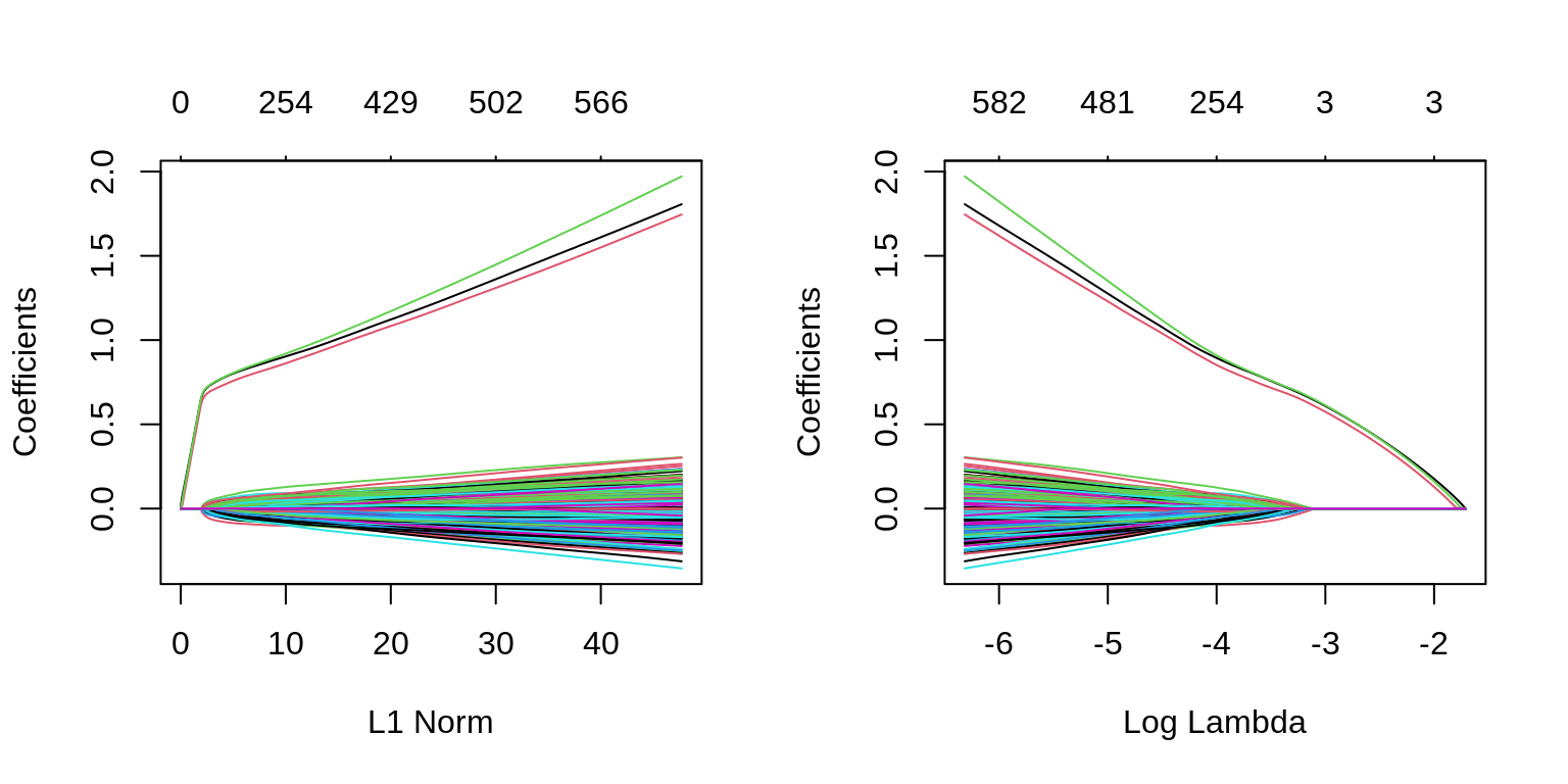
We can extract the two relevant \(\lambda\) values.
## [1] 0.03718493## [1] 0.0514969Since cv.glmnet() does not calculate prediction accuracy for classification, we take the \(\lambda\) values and create a grid for caret to search in order to obtain prediction accuracy with train(). We set \(\alpha = 1\) in this grid, as glmnet can actually tune over the \(\alpha = 1\) parameter. (More on that later.)
Note that we have to force y to be a factor, so that train() recognizes we want to have a binomial response. The train() function in caret use the type of variable in y to determine if you want to use family = "binomial" or family = "gaussian".
library(caret)
cv_5 = trainControl(method = "cv", number = 5)
lasso_grid = expand.grid(alpha = 1,
                         lambda = c(fit_cv$lambda.min, fit_cv$lambda.1se))
lasso_grid
## alpha lambda
## 1 1 0.03718493
## 2 1 0.05149690sim_data = data.frame(y, X)
fit_lasso = train(
y ~ ., data = sim_data,
method = "glmnet",
trControl = cv_5,
tuneGrid = lasso_grid
)
fit_lasso$results## alpha lambda Accuracy Kappa AccuracySD KappaSD
## 1 1 0.03718493 0.7560401 0.5119754 0.01738219 0.03459404
## 2 1 0.05149690 0.7690353 0.5380106 0.02166057 0.04323249The interaction between the glmnet and caret packages is sometimes frustrating, but for obtaining results for particular values of \(\lambda\), we see it can be easily used. More on this next chapter.
24.5 External Links
glmnetWeb Vingette - Details from the package developers.
24.6 rmarkdown
The rmarkdown file for this chapter can be found here. The file was created using R version 4.0.2. The following packages (and their dependencies) were loaded when knitting this file:
## [1] "caret" "ggplot2" "lattice" "broom" "glmnet" "Matrix"