Chapter 14 Shrinkage Methods
We will use the Hitters dataset from the ISLR package to explore two shrinkage methods: ridge and lasso. These are otherwise known as penalized regression methods.
data(Hitters, package = "ISLR")This dataset has some missing data in the response Salaray. We use the na.omit() function the clean the dataset.
sum(is.na(Hitters))## [1] 59sum(is.na(Hitters$Salary))## [1] 59Hitters = na.omit(Hitters)
sum(is.na(Hitters))## [1] 0The predictors variables are offensive and defensive statistics for a number of baseball players.
names(Hitters)## [1] "AtBat" "Hits" "HmRun" "Runs" "RBI"
## [6] "Walks" "Years" "CAtBat" "CHits" "CHmRun"
## [11] "CRuns" "CRBI" "CWalks" "League" "Division"
## [16] "PutOuts" "Assists" "Errors" "Salary" "NewLeague"We use the glmnet() and cv.glmnet() functions in the glmnet package to fit penalized regressions.
# this is a temporary workaround for an issue with glmnet, Matrix, and R version 3.3.3
# see here: http://stackoverflow.com/questions/43282720/r-error-in-validobject-object-when-running-as-script-but-not-in-console
library(methods)library(glmnet)The glmnet function does not allow the use of model formulas, so we setup the data for ease of use with glmnet.
X = model.matrix(Salary ~ ., Hitters)[, -1]
y = Hitters$Salary
First, we fit a regular linear regression, and note the size of the predictors’ coefficients, and predictors’ coefficients squared. (The two penalties we will use.)
fit = lm(Salary ~ ., Hitters)
coef(fit)
## (Intercept) AtBat Hits HmRun Runs
## 163.1035878 -1.9798729 7.5007675 4.3308829 -2.3762100
## RBI Walks Years CAtBat CHits
## -1.0449620 6.2312863 -3.4890543 -0.1713405 0.1339910
## CHmRun CRuns CRBI CWalks LeagueN
## -0.1728611 1.4543049 0.8077088 -0.8115709 62.5994230
## DivisionW PutOuts Assists Errors NewLeagueN
## -116.8492456 0.2818925 0.3710692 -3.3607605 -24.7623251sum(abs(coef(fit)[-1]))## [1] 238.7295sum(coef(fit)[-1] ^ 2)## [1] 18337.314.1 Ridge Regression
We first illustrate ridge regression, which can be fit using glmnet() with alpha = 0 and seeks to minimize
\[ \sum_{i=1}^{n} \left( y_i - \beta_0 - \sum_{j=1}^{p} \beta_j x_{ij} \right) ^ 2 + \lambda \sum_{j=1}^{p} \beta_j^2 . \]
Notice that the intercept is not penalized. Also, note that that ridge regression is not scale invariant like the usual unpenalized regression. Thankfully, glmnet() takes care of this internally. It automatically standardizes input for fitting, then reports fitted coefficient using the original scale.
The two plots illustrate how much the coefficients are penalized for different values of \(\lambda\). Notice none of the coefficients are forced to be zero.
fit_ridge = glmnet(X, y, alpha = 0)
plot(fit_ridge)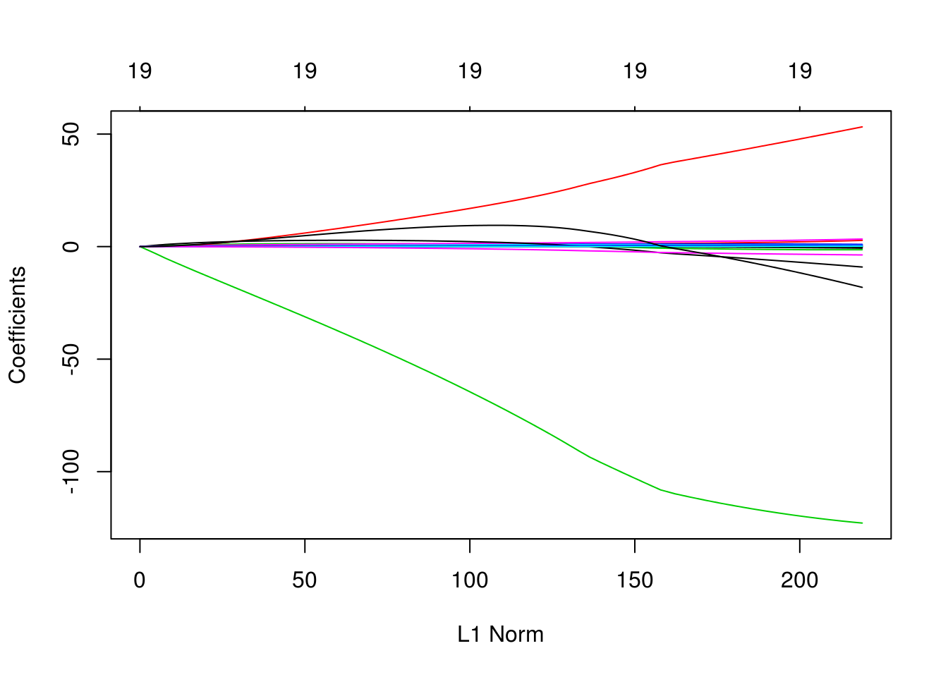
plot(fit_ridge, xvar = "lambda", label = TRUE)
dim(coef(fit_ridge))## [1] 20 100We use cross-validation to select a good \(\lambda\) value. The cv.glmnet()function uses 10 folds by default. The plot illustrates the MSE for the \(\lambda\)s considered. Two lines are drawn. The first is the \(\lambda\) that gives the smallest MSE. The second is the \(\lambda\) that gives an MSE within one standard error of the smallest.
fit_ridge_cv = cv.glmnet(X, y, alpha = 0)
plot(fit_ridge_cv)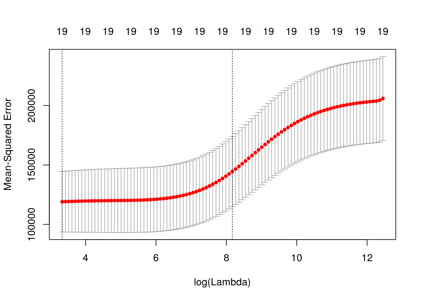
The cv.glmnet() function returns several details of the fit for both \(\lambda\) values in the plot. Notice the penalty terms are smaller than the full linear regression. (As we would expect.)
coef(fit_ridge_cv)## 20 x 1 sparse Matrix of class "dgCMatrix"
## 1
## (Intercept) 254.518230141
## AtBat 0.079408204
## Hits 0.317375220
## HmRun 1.065097243
## Runs 0.515835607
## RBI 0.520504723
## Walks 0.661891621
## Years 2.231379426
## CAtBat 0.006679258
## CHits 0.025455999
## CHmRun 0.189661478
## CRuns 0.051057906
## CRBI 0.052776153
## CWalks 0.052170266
## LeagueN 2.114989228
## DivisionW -17.479743519
## PutOuts 0.043039515
## Assists 0.006296277
## Errors -0.099487300
## NewLeagueN 2.085946064coef(fit_ridge_cv, s = "lambda.min")## 20 x 1 sparse Matrix of class "dgCMatrix"
## 1
## (Intercept) 7.645824e+01
## AtBat -6.315180e-01
## Hits 2.642160e+00
## HmRun -1.388233e+00
## Runs 1.045729e+00
## RBI 7.315713e-01
## Walks 3.278001e+00
## Years -8.723734e+00
## CAtBat 1.256354e-04
## CHits 1.318975e-01
## CHmRun 6.895578e-01
## CRuns 2.830055e-01
## CRBI 2.514905e-01
## CWalks -2.599851e-01
## LeagueN 5.233720e+01
## DivisionW -1.224170e+02
## PutOuts 2.623667e-01
## Assists 1.629044e-01
## Errors -3.644002e+00
## NewLeagueN -1.702598e+01sum(coef(fit_ridge_cv, s = "lambda.min")[-1] ^ 2) # penalty term for lambda minimum## [1] 18126.85coef(fit_ridge_cv, s = "lambda.1se")## 20 x 1 sparse Matrix of class "dgCMatrix"
## 1
## (Intercept) 254.518230141
## AtBat 0.079408204
## Hits 0.317375220
## HmRun 1.065097243
## Runs 0.515835607
## RBI 0.520504723
## Walks 0.661891621
## Years 2.231379426
## CAtBat 0.006679258
## CHits 0.025455999
## CHmRun 0.189661478
## CRuns 0.051057906
## CRBI 0.052776153
## CWalks 0.052170266
## LeagueN 2.114989228
## DivisionW -17.479743519
## PutOuts 0.043039515
## Assists 0.006296277
## Errors -0.099487300
## NewLeagueN 2.085946064sum(coef(fit_ridge_cv, s = "lambda.1se")[-1] ^ 2) # penalty term for lambda one SE## [1] 321.618#predict(fit_ridge_cv, X, s = "lambda.min")
#predict(fit_ridge_cv, X)
mean((y - predict(fit_ridge_cv, X)) ^ 2) # "train error"## [1] 138732.7sqrt(fit_ridge_cv$cvm) # CV-RMSEs## [1] 453.8860 452.3053 451.4592 451.1916 450.8992 450.5796 450.2305
## [8] 449.8494 449.4336 448.9802 448.4860 447.9478 447.3619 446.7248
## [15] 446.0326 445.2809 444.4659 443.5831 442.6278 441.5957 440.4821
## [22] 439.2823 437.9920 436.6068 435.1226 433.5357 431.8430 430.0418
## [29] 428.1303 426.1075 423.9734 421.7292 419.3776 416.9224 414.3693
## [36] 411.7254 408.9996 406.2020 403.3448 400.4415 397.5070 394.5572
## [43] 391.6087 388.6788 385.7846 382.9431 380.1704 377.4818 374.8911
## [50] 372.4100 370.0477 367.8126 365.7110 363.7462 361.9197 360.2309
## [57] 358.6776 357.2562 355.9618 354.7883 353.7293 352.7775 351.9259
## [64] 351.1642 350.4893 349.8946 349.3717 348.9146 348.5131 348.1695
## [71] 347.8752 347.6187 347.4060 347.2272 347.0712 346.9474 346.8403
## [78] 346.7540 346.6785 346.6202 346.5660 346.5176 346.4743 346.4268
## [85] 346.3808 346.3309 346.2774 346.2170 346.1518 346.0767 345.9918
## [92] 345.9048 345.8043 345.6976 345.5829 345.4590 345.3311 345.1996
## [99] 345.0604sqrt(fit_ridge_cv$cvm[fit_ridge_cv$lambda == fit_ridge_cv$lambda.min]) # CV-RMSE minimum## [1] 345.0604sqrt(fit_ridge_cv$cvm[fit_ridge_cv$lambda == fit_ridge_cv$lambda.1se]) # CV-RMSE one SE## [1] 380.170414.2 Lasso
We now illustrate lasso, which can be fit using glmnet() with alpha = 1 and seeks to minimize
\[ \sum_{i=1}^{n} \left( y_i - \beta_0 - \sum_{j=1}^{p} \beta_j x_{ij} \right) ^ 2 + \lambda \sum_{j=1}^{p} |\beta_j| . \]
Like ridge, lasso is not scale invariant.
The two plots illustrate how much the coefficients are penalized for different values of \(\lambda\). Notice some of the coefficients are forced to be zero.
fit_lasso = glmnet(X, y, alpha = 1)
plot(fit_lasso)
plot(fit_lasso, xvar = "lambda", label = TRUE)
dim(coef(fit_lasso))## [1] 20 80Again, to actually pick a \(\lambda\), we will use cross-validation. The plot is similar to the ridge plot. Notice along the top is the number of features in the model. (Which changed in this plot.)
fit_lasso_cv = cv.glmnet(X, y, alpha = 1)
plot(fit_lasso_cv)
cv.glmnet() returns several details of the fit for both \(\lambda\) values in the plot. Notice the penalty terms are again smaller than the full linear regression. (As we would expect.) Some coefficients are 0.
coef(fit_lasso_cv)## 20 x 1 sparse Matrix of class "dgCMatrix"
## 1
## (Intercept) 167.91202818
## AtBat .
## Hits 1.29269756
## HmRun .
## Runs .
## RBI .
## Walks 1.39817511
## Years .
## CAtBat .
## CHits .
## CHmRun .
## CRuns 0.14167760
## CRBI 0.32192558
## CWalks .
## LeagueN .
## DivisionW .
## PutOuts 0.04675463
## Assists .
## Errors .
## NewLeagueN .coef(fit_lasso_cv, s = "lambda.min")## 20 x 1 sparse Matrix of class "dgCMatrix"
## 1
## (Intercept) 129.4155571
## AtBat -1.6130155
## Hits 5.8058915
## HmRun .
## Runs .
## RBI .
## Walks 4.8469340
## Years -9.9724045
## CAtBat .
## CHits .
## CHmRun 0.5374550
## CRuns 0.6811938
## CRBI 0.3903563
## CWalks -0.5560144
## LeagueN 32.4646094
## DivisionW -119.3480842
## PutOuts 0.2741895
## Assists 0.1855978
## Errors -2.1650837
## NewLeagueN .sum(abs(coef(fit_lasso_cv, s = "lambda.min")[-1])) # penalty term for lambda minimum## [1] 178.8408coef(fit_lasso_cv, s = "lambda.1se")## 20 x 1 sparse Matrix of class "dgCMatrix"
## 1
## (Intercept) 167.91202818
## AtBat .
## Hits 1.29269756
## HmRun .
## Runs .
## RBI .
## Walks 1.39817511
## Years .
## CAtBat .
## CHits .
## CHmRun .
## CRuns 0.14167760
## CRBI 0.32192558
## CWalks .
## LeagueN .
## DivisionW .
## PutOuts 0.04675463
## Assists .
## Errors .
## NewLeagueN .sum(abs(coef(fit_lasso_cv, s = "lambda.1se")[-1])) # penalty term for lambda one SE## [1] 3.20123#predict(fit_lasso_cv, X, s = "lambda.min")
#predict(fit_lasso_cv, X)
mean((y - predict(fit_lasso_cv, X)) ^ 2) # "train error"## [1] 123931.3sqrt(fit_lasso_cv$cvm)## [1] 450.4667 439.5342 429.1014 420.2278 411.7974 403.1526 395.2030
## [8] 388.1047 381.8172 376.4784 371.9706 367.9954 364.6244 361.8324
## [15] 359.0267 355.8590 352.9123 350.4139 348.3320 346.5990 345.1582
## [22] 343.9776 343.0062 342.2064 341.6185 341.1848 341.0257 341.0220
## [29] 341.0680 341.1822 341.3420 341.5010 341.6557 341.8143 341.9259
## [36] 342.0843 342.4935 342.7806 342.5019 341.8506 341.0687 340.2737
## [43] 339.5857 339.0583 338.4835 337.8989 337.4145 337.1080 336.8034
## [50] 336.6050 336.4913 336.5493 336.6815 336.8781 336.9805 337.0503
## [57] 337.1468 337.1720 337.1742 337.2114 337.3021 337.4978 337.7147
## [64] 337.9278 338.1234 338.3568 338.5477 338.7480 338.9406 339.1208
## [71] 339.2701 339.4129 339.5202 339.6048sqrt(fit_lasso_cv$cvm[fit_lasso_cv$lambda == fit_lasso_cv$lambda.min]) # CV-RMSE minimum## [1] 336.4913sqrt(fit_lasso_cv$cvm[fit_lasso_cv$lambda == fit_lasso_cv$lambda.1se]) # CV-RMSE one SE## [1] 364.624414.3 broom
Sometimes, the output from glmnet() can be overwhelming. The broom package can help with that.
library(broom)
#fit_lasso_cv
tidy(fit_lasso_cv)
## lambda estimate std.error conf.high conf.low nzero
## 1 255.2820965 202920.3 25218.50 228138.8 177701.78 0
## 2 232.6035386 193190.3 25203.86 218394.2 167986.46 1
## 3 211.9396813 184128.0 24929.00 209057.0 159199.04 2
## 4 193.1115442 176591.4 24686.50 201277.9 151904.87 2
## 5 175.9560468 169577.1 24414.65 193991.7 145162.42 3
## 6 160.3245966 162532.0 24377.15 186909.2 138154.87 4
## 7 146.0818013 156185.4 24257.32 180442.7 131928.08 4
## 8 133.1042967 150625.2 24049.18 174674.4 126576.05 4
## 9 121.2796778 145784.4 23808.60 169593.0 121975.81 4
## 10 110.5055255 141736.0 23620.54 165356.5 118115.44 4
## 11 100.6885192 138362.1 23502.45 161864.6 114859.65 5
## 12 91.7436287 135420.6 23435.61 158856.2 111984.99 5
## 13 83.5933775 132951.0 23398.99 156350.0 109551.97 5
## 14 76.1671723 130922.7 23398.34 154321.0 107524.35 5
## 15 69.4006906 128900.2 23437.48 152337.7 105462.72 6
## 16 63.2353245 126635.6 23389.74 150025.4 103245.89 6
## 17 57.6176726 124547.1 23291.03 147838.1 101256.07 6
## 18 52.4990774 122789.9 23206.06 145996.0 99583.87 6
## 19 47.8352040 121335.2 23140.34 144475.5 98194.84 6
## 20 43.5856563 120130.8 23089.89 143220.7 97040.94 6
## 21 39.7136268 119134.2 23053.48 142187.7 96080.72 6
## 22 36.1855776 118320.6 23029.81 141350.4 95290.80 6
## 23 32.9709506 117653.2 23014.34 140667.6 94638.88 6
## 24 30.0419022 117105.2 23004.92 140110.2 94100.30 6
## 25 27.3730624 116703.2 23008.15 139711.4 93695.05 6
## 26 24.9413150 116407.1 23019.55 139426.6 93387.53 6
## 27 22.7255973 116298.5 23114.05 139412.6 93184.45 6
## 28 20.7067179 116296.0 23191.03 139487.1 93105.01 6
## 29 18.8671902 116327.4 23258.64 139586.0 93068.72 6
## 30 17.1910810 116405.3 23321.28 139726.6 93084.03 7
## 31 15.6638727 116514.3 23381.61 139895.9 93132.72 7
## 32 14.2723374 116623.0 23440.59 140063.5 93182.37 7
## 33 13.0044223 116728.6 23496.59 140225.2 93232.00 9
## 34 11.8491453 116837.0 23547.75 140384.7 93289.24 9
## 35 10.7964999 116913.3 23585.20 140498.5 93328.12 9
## 36 9.8373686 117021.6 23626.34 140648.0 93395.30 9
## 37 8.9634439 117301.8 23647.80 140949.6 93654.02 9
## 38 8.1671562 117498.5 23683.21 141181.7 93815.30 11
## 39 7.4416086 117307.6 23571.59 140879.2 93735.97 11
## 40 6.7805166 116861.8 23398.00 140259.8 93463.83 12
## 41 6.1781542 116327.8 23218.01 139545.9 93109.83 12
## 42 5.6293040 115786.2 23055.36 138841.5 92730.82 13
## 43 5.1292121 115318.4 22913.69 138232.1 92404.75 13
## 44 4.6735471 114960.5 22802.85 137763.4 92157.66 13
## 45 4.2583620 114571.1 22691.64 137262.7 91879.46 13
## 46 3.8800609 114175.7 22554.23 136729.9 91621.46 13
## 47 3.5353670 113848.5 22418.32 136266.8 91430.21 13
## 48 3.2212947 113641.8 22283.59 135925.4 91358.24 13
## 49 2.9351238 113436.5 22169.36 135605.9 91267.14 13
## 50 2.6743755 113302.9 22065.47 135368.4 91237.43 13
## 51 2.4367913 113226.4 21990.47 135216.9 91235.92 13
## 52 2.2203135 113265.4 21912.06 135177.5 91353.38 14
## 53 2.0230670 113354.4 21845.22 135199.7 91509.22 15
## 54 1.8433433 113486.9 21789.57 135276.4 91697.30 15
## 55 1.6795857 113555.8 21723.84 135279.7 91832.00 17
## 56 1.5303760 113602.9 21675.98 135278.9 91926.92 17
## 57 1.3944216 113668.0 21643.70 135311.7 92024.29 17
## 58 1.2705450 113685.0 21620.15 135305.1 92064.83 17
## 59 1.1576733 113686.5 21593.07 135279.5 92093.40 17
## 60 1.0548288 113711.6 21573.64 135285.2 92137.92 17
## 61 0.9611207 113772.7 21561.10 135333.8 92211.58 17
## 62 0.8757374 113904.8 21548.51 135453.3 92356.24 17
## 63 0.7979393 114051.2 21537.17 135588.4 92514.06 17
## 64 0.7270526 114195.2 21517.33 135712.5 92677.88 17
## 65 0.6624632 114327.4 21501.10 135828.5 92826.33 18
## 66 0.6036118 114485.3 21484.99 135970.3 93000.31 18
## 67 0.5499886 114614.6 21472.42 136087.0 93142.13 18
## 68 0.5011291 114750.2 21459.91 136210.1 93290.27 17
## 69 0.4566102 114880.7 21448.88 136329.6 93431.86 18
## 70 0.4160462 115002.9 21450.62 136453.5 93552.26 18
## 71 0.3790858 115104.2 21452.03 136556.2 93652.17 18
## 72 0.3454089 115201.1 21452.72 136653.8 93748.38 18
## 73 0.3147237 115274.0 21457.78 136731.8 93816.22 18
## 74 0.2867645 115331.4 21461.84 136793.2 93869.57 18glance(fit_lasso_cv) # the two lambda values of interest## lambda.min lambda.1se
## 1 2.436791 83.5933814.4 Simulation Study, p > n
Aside from simply shrinking coefficients (ridge) and setting some coefficients to 0 (lasso), penalized regression also has the advantage of being able to handle the \(p > n\) case.
set.seed(1234)
n = 1000
p = 5500
X = replicate(p, rnorm(n = n))
beta = c(1, 1, 1, rep(0, 5497))
z = X %*% beta
prob = exp(z) / (1 + exp(z))
y = as.factor(rbinom(length(z), size = 1, prob = prob))
We first simulate a classification example where \(p > n\).
# glm(y ~ X, family = "binomial")
# will not converge
We then use a lasso penalty to fit penalized logistic regression. This minimizes
\[ \sum_{i=1}^{n} L\left(y_i, \beta_0 + \sum_{j=1}^{p} \beta_j x_{ij}\right) + \lambda \sum_{j=1}^{p} |\beta_j| \]
where \(L\) is the appropriate negative log-likelihood.
library(glmnet)
fit_cv = cv.glmnet(X, y, family = "binomial", alpha = 1)
plot(fit_cv)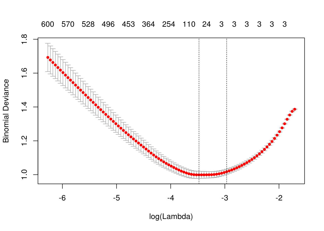
head(coef(fit_cv), n = 10)## 10 x 1 sparse Matrix of class "dgCMatrix"
## 1
## (Intercept) 0.02397452
## V1 0.59674958
## V2 0.56251761
## V3 0.60065105
## V4 .
## V5 .
## V6 .
## V7 .
## V8 .
## V9 .fit_cv$nzero## s0 s1 s2 s3 s4 s5 s6 s7 s8 s9 s10 s11 s12 s13 s14 s15 s16 s17
## 0 2 3 3 3 3 3 3 3 3 3 3 3 3 3 3 3 3
## s18 s19 s20 s21 s22 s23 s24 s25 s26 s27 s28 s29 s30 s31 s32 s33 s34 s35
## 3 3 3 3 3 3 3 3 3 3 3 3 4 6 7 10 18 24
## s36 s37 s38 s39 s40 s41 s42 s43 s44 s45 s46 s47 s48 s49 s50 s51 s52 s53
## 35 54 65 75 86 100 110 129 147 168 187 202 221 241 254 269 283 298
## s54 s55 s56 s57 s58 s59 s60 s61 s62 s63 s64 s65 s66 s67 s68 s69 s70 s71
## 310 324 333 350 364 375 387 400 411 429 435 445 453 455 462 466 475 481
## s72 s73 s74 s75 s76 s77 s78 s79 s80 s81 s82 s83 s84 s85 s86 s87 s88 s89
## 487 491 496 498 502 504 512 518 523 526 528 536 543 550 559 561 563 566
## s90 s91 s92 s93 s94 s95 s96 s97 s98
## 570 571 576 582 586 590 596 596 600Notice, only the first three predictors generated are truly significant, and that is exactly what the suggested model finds.
fit_1se = glmnet(X, y, family = "binomial", lambda = fit_cv$lambda.1se)
which(as.vector(as.matrix(fit_1se$beta)) != 0)
## [1] 1 2 3We can also see in the following plots, the three features entering the model well ahead of the irrelevant features.
plot(glmnet(X, y, family = "binomial"))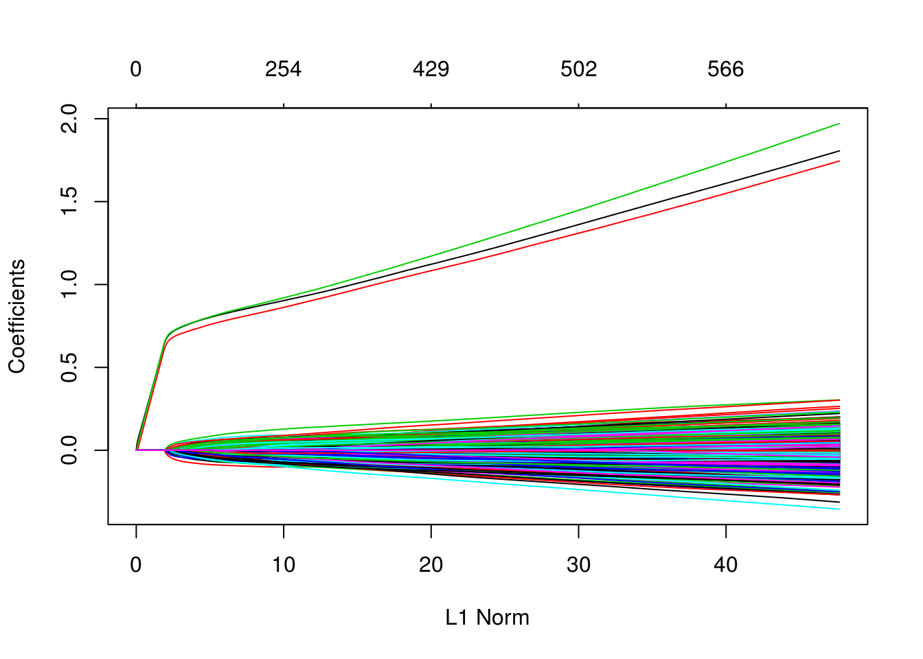
plot(glmnet(X, y, family = "binomial"), xvar = "lambda")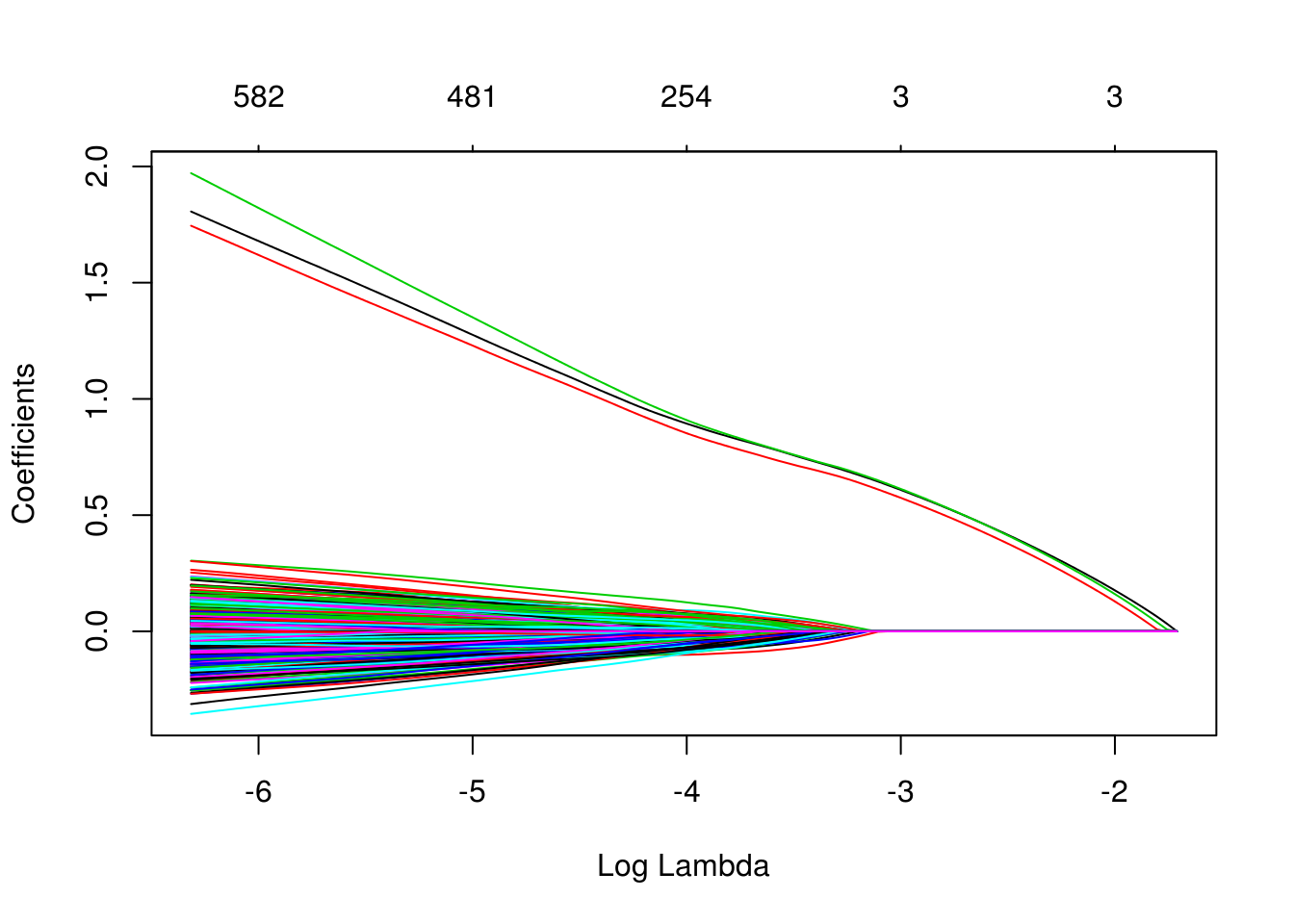
We can extract the two relevant \(\lambda\) values.
fit_cv$lambda.min## [1] 0.03087158fit_cv$lambda.1se## [1] 0.0514969Since cv.glmnet() does not calculate prediction accuracy for classification, we take the \(\lambda\) values and create a grid for caret to search in order to obtain prediction accuracy with train(). We set \(\alpha = 1\) in this grid, as glmnet can actually tune over the \(\alpha = 1\) parameter. (More on that later.)
Note that we have to force y to be a factor, so that train() recognizes we want to have a binomial response. The train() function in caret use the type of variable in y to determine if you want to use family = "binomial" or family = "gaussian".
library(caret)
cv_5 = trainControl(method = "cv", number = 5)
lasso_grid = expand.grid(alpha = 1,
                         lambda = c(fit_cv$lambda.min, fit_cv$lambda.1se))
lasso_grid
## alpha lambda
## 1 1 0.03087158
## 2 1 0.05149690sim_data = data.frame(y, X)
fit_lasso = train(
y ~ ., data = sim_data,
method = "glmnet",
trControl = cv_5,
tuneGrid = lasso_grid
)
fit_lasso$results## alpha lambda Accuracy Kappa AccuracySD KappaSD
## 1 1 0.03087158 0.7609903 0.5218887 0.01486223 0.03000986
## 2 1 0.05149690 0.7659604 0.5319189 0.01807380 0.0359431914.5 External Links
glmnetWeb Vingette - Details from the package developers.
14.6 RMarkdown
The RMarkdown file for this chapter can be found here. The file was created using R version 3.4.1 and the following packages:
- Base Packages, Attached
## [1] "methods"   "stats"     "graphics"  "grDevices" "utils"     "datasets"
## [7] "base"- Additional Packages, Attached
## [1] "caret" "ggplot2" "lattice" "broom" "glmnet" "foreach" "Matrix"- Additional Packages, Not Attached
##  [1] "reshape2"     "splines"      "colorspace"   "htmltools"
##  [5] "stats4"       "yaml"         "mgcv"         "rlang"
##  [9] "ModelMetrics" "e1071"        "nloptr"       "foreign"
## [13] "glue"         "bindrcpp"     "bindr"        "plyr"
## [17] "stringr"      "MatrixModels" "munsell"      "gtable"
## [21] "codetools"    "psych"        "evaluate"     "knitr"
## [25] "SparseM"      "class"        "quantreg"     "pbkrtest"
## [29] "parallel"     "Rcpp"         "backports"    "scales"
## [33] "lme4"         "mnormt"       "digest"       "stringi"
## [37] "bookdown"     "dplyr"        "grid"         "rprojroot"
## [41] "tools"        "magrittr"     "lazyeval"     "tibble"
## [45] "tidyr"        "car"          "pkgconfig"    "MASS"
## [49] "assertthat"   "minqa"        "rmarkdown"    "iterators"
## [53] "R6"           "nnet"         "nlme"         "compiler"