Chapter 8 Simulation
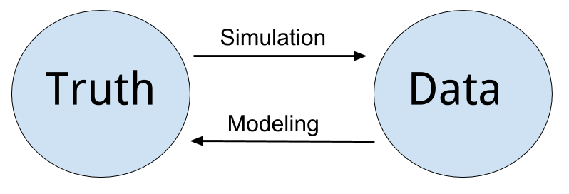
Simulation and model fitting are related but opposite processes.
- In simulation, the data generating process is known. We will know the form of the model as well as the value of each of the parameters. In particular, we will often control the distribution and parameters which define the randomness, or noise in the data.
- In model fitting, the data is known. We will then assume a certain form of model and find the best possible values of the parameters given the observed data. Essentially we are seeking to uncover the truth. Often we will attempt to fit many models, and we will learn metrics to assess which model fits best.

Simulation vs Modeling
Often we will simulate data according to a process we decide, then use a modeling method seen in class. We can then verify how well the method works, since we know the data generating process.
One of the biggest strengths of R is its ability to carry out simulations using built-in functions for generating random samples from certain distributions. We’ll look at two very simple examples here, however simulation will be a topic we revisit several times throughout the course.
8.0.1 Paired Differences
Consider the model:
\[ \begin{split} X_{11}, X_{12}, \ldots, X_{1n} \sim N(\mu_1,\sigma^2)\\ X_{21}, X_{22}, \ldots, X_{2n} \sim N(\mu_2,\sigma^2) \end{split} \]
Assume that \(\mu_1 = 6\), \(\mu_2 = 5\), \(\sigma^2 = 4\) and \(n = 25\).
Let
\[ \begin{aligned} \bar{X}_1 &= \displaystyle\frac{1}{n}\sum_{i=1}^{n}X_{1i}\\ \bar{X}_2 &= \displaystyle\frac{1}{n}\sum_{i=1}^{n}X_{2i}\\ D &= \bar{X}_1 - \bar{X}_2. \end{aligned} \]
Suppose we would like to calculate \(P(0 < D < 2)\). First we will need to obtain the distribution of \(D\).
Recall,
\[ \bar{X}_1 \sim N\left(\mu_1,\frac{\sigma^2}{n}\right) \]
and
\[ \bar{X}_2 \sim N\left(\mu_2,\frac{\sigma^2}{n}\right). \]
Then,
\[ D = \bar{X}_1 - \bar{X}_2 \sim N\left(\mu_1-\mu_2, \frac{\sigma^2}{n} + \frac{\sigma^2}{n}\right) = N\left(6-5, \frac{4}{25} + \frac{4}{25}\right). \]
So,
\[ D \sim N(\mu = 1, \sigma^2 = 0.32). \]
Thus,
\[ P(0 < D < 2) = P(D < 2) - P(D < 0). \]
This can then be calculated using R without a need to first standardize, or use a table.
pnorm(2, mean = 1, sd = sqrt(0.32)) - pnorm(0, mean = 1, sd = sqrt(0.32))## [1] 0.9229001An alternative approach, would be to simulate a large number of observations of \(D\) then use the empirical distribution to calculate the probability.
Our strategy will be to repeatedly:
- Generate a sample of 25 random observations from \(N(\mu_1 = 6,\sigma^2 = 4)\). Call the mean of this sample \(\bar{x}_{1s}\).
- Generate a sample of 25 random observations from \(N(\mu_1 = 5,\sigma^2 = 4)\). Call the mean of this sample \(\bar{x}_{2s}\).
- Calculate the differences of the means, \(d_s = \bar{x}_{1s} - \bar{x}_{2s}\).
We will repeat the process a large number of times. Then we will use the distribution of the simulated observations of \(d_s\) as an estimate for the true distribution of \(D\).
set.seed(42)
num_samples = 10000
differences = rep(0, num_samples)
Before starting our for loop to perform the operation, we set a seed for reproducibility, create and set a variable num_samples which will define the number of repetitions, and lastly create a variables differences which will store the simulate values, \(d_s\).
By using set.seed() we can reproduce the random results of rnorm() each time starting from that line.
for (s in 1:num_samples) {
  x1 = rnorm(n = 25, mean = 6, sd = 2)
  x2 = rnorm(n = 25, mean = 5, sd = 2)
  differences[s] = mean(x1) - mean(x2)
}
To estimate \(P(0 < D < 2)\) we will find the proportion of values of \(d_s\) (among the 10^{4} values of \(d_s\) generated) that are between 0 and 2.
mean(0 < differences & differences < 2)## [1] 0.9222Recall that above we derived the distribution of \(D\) to be \(N(\mu = 1, \sigma^2 = 0.32)\)
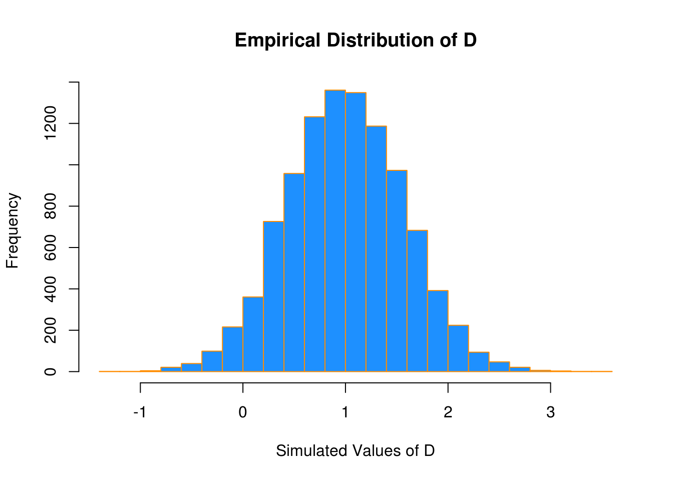
If we look at a histogram of the differences, we find that it looks very much like a normal distribution.
hist(differences, breaks = 20,
     main   = "Empirical Distribution of D",
     xlab   = "Simulated Values of D",
     col    = "dodgerblue",
     border = "darkorange")
Also the sample mean and variance are very close to to what we would expect.
mean(differences)## [1] 1.001423var(differences)## [1] 0.3230183We could have also accomplished this task with a single line of more “idiomatic” R.
set.seed(42)
diffs = replicate(10000, mean(rnorm(25, 6, 2)) - mean(rnorm(25, 5, 2)))
Use ?replicate to take a look at the documentation for the replicate function and see if you can understand how this line performs the same operations that our for loop above executed.
mean(differences == diffs)## [1] 1We see that by setting the same seed for the randomization, we actually obtain identical results!
8.0.2 Distribution of a Sample Mean
For another example of simulation, we will simulate observations from a Poisson distribution, and examine the empirical distribution of the sample mean of these observations.
Recall, if
\[ X \sim Pois(\mu) \]
then
\[ E[X] = \mu \]
and
\[ Var[X] = \mu. \]
Also, recall that for a random variable \(X\) with finite mean \(\mu\) and finite variance \(\sigma^2\), the central limit theorem tells us that the mean, \(\bar{X}\) of a random sample of size \(n\) is approximately normal for large values of \(n\). Specifically, as \(n \to \infty\),
\[ \bar{X} \overset{d}{\to} N\left(\mu, \frac{\sigma^2}{n}\right). \]
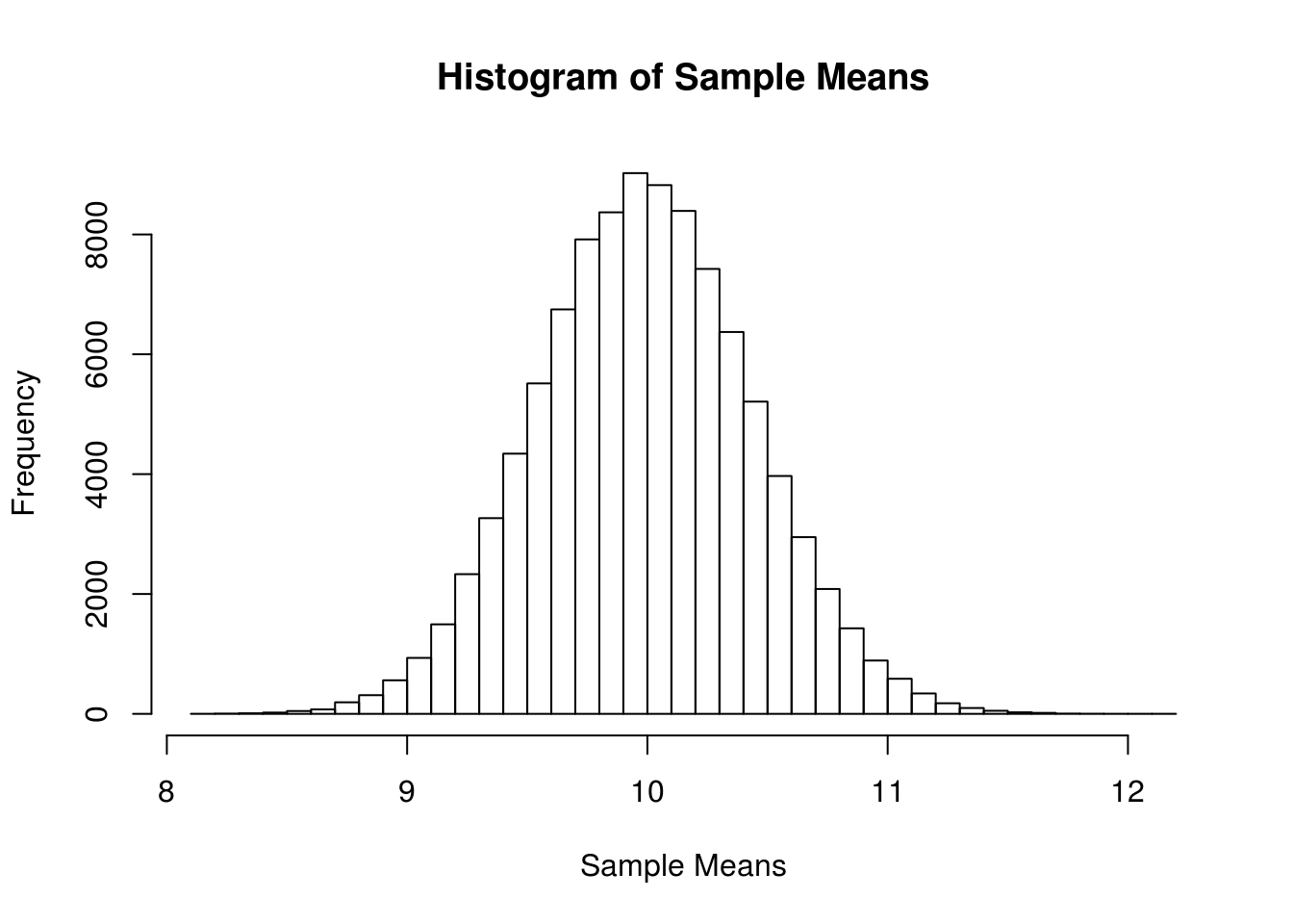
The following verifies this result for a Poisson distribution with \(\mu = 10\) and a sample size of \(n = 50\).
set.seed(1337)
mu          = 10
sample_size = 50
samples     = 100000
x_bars      = rep(0, samples)
for(i in 1:samples){
x_bars[i] = mean(rpois(sample_size, lambda = mu))
}x_bar_hist = hist(x_bars, breaks = 50,
main = "Histogram of Sample Means",
xlab = "Sample Means")
Now we will compare sample statistics from the empirical distribution with their known values based on the parent distribution.
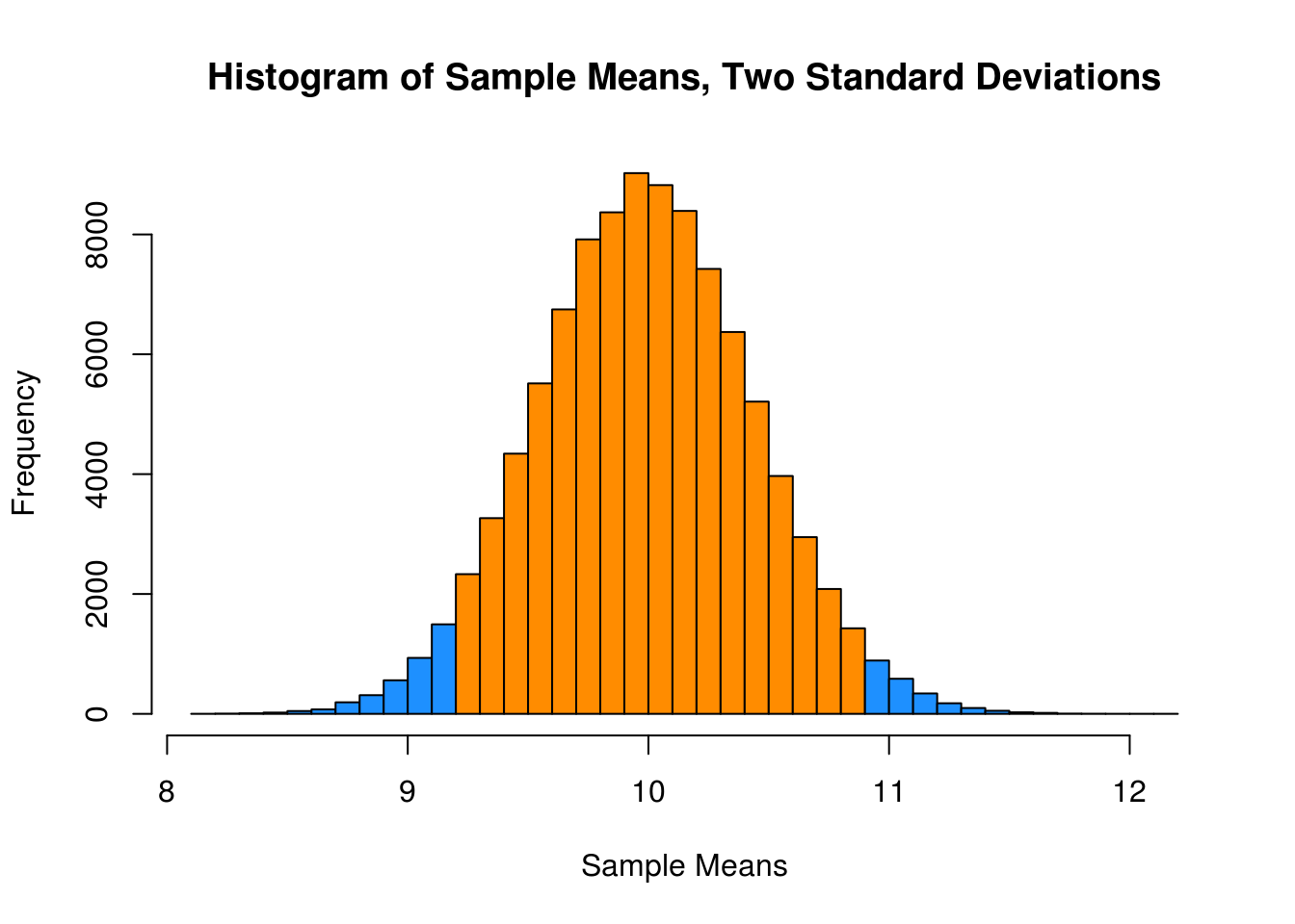
c(mean(x_bars), mu)## [1] 10.00008 10.00000c(var(x_bars), mu / sample_size)## [1] 0.1989732 0.2000000c(sd(x_bars), sqrt(mu) / sqrt(sample_size))## [1] 0.4460641 0.4472136And here, we will calculate the proportion of sample means that are within 2 standard deviations of the population mean.
mean(x_bars > mu - 2 * sqrt(mu) / sqrt(sample_size) &
     x_bars < mu + 2 * sqrt(mu) / sqrt(sample_size))
## [1] 0.95429This last histogram uses a bit of a trick to approximately shade the bars that are within two standard deviations of the mean.)
shading = ifelse(x_bar_hist$breaks > mu - 2 * sqrt(mu) / sqrt(sample_size) &
                   x_bar_hist$breaks < mu + 2 * sqrt(mu) / sqrt(sample_size),
                  "darkorange", "dodgerblue")

x_bar_hist = hist(x_bars, breaks = 50, col = shading,
                  main = "Histogram of Sample Means, Two Standard Deviations",
                  xlab = "Sample Means")